Problem Statement:
A retail company “ABC Private Limited” wants to understand the customer purchase behaviour (specifically, purchase amount) against various products of different categories. They have shared purchase summary of various customers for selected high volume products from last month. The data set also contains customer demographics (age, gender, marital status, city_type, stay_in_current_city), product details (product_id and product category) and Total purchase_amount from last month.
Now, they want to build a model to predict the purchase amount of customer against various products which will help them to create personalized offer for customers against different products. The dataset can be found here.
The dataset already consists of a train set and a test set.
What we will be doing is preparing the data for modeling.
import pandas as pd
import numpy as np
import matplotlib
import matplotlib.pyplot as plt
import seaborn as sns
%matplotlib inline

matplotlib.rcParams['figure.figsize'] = (12, 6)
pd.set_option('display.max_columns', None)
# import the train dataset
df_train = pd.read_csv('data/black_friday/train.csv')
df_train.head()| User_ID | Product_ID | Gender | Age | Occupation | City_Category | Stay_In_Current_City_Years | Marital_Status | Product_Category_1 | Product_Category_2 | Product_Category_3 | Purchase | |
|---|---|---|---|---|---|---|---|---|---|---|---|---|
| 0 | 1000001 | P00069042 | F | 0-17 | 10 | A | 2 | 0 | 3 | NaN | NaN | 8370 |
| 1 | 1000001 | P00248942 | F | 0-17 | 10 | A | 2 | 0 | 1 | 6.0 | 14.0 | 15200 |
| 2 | 1000001 | P00087842 | F | 0-17 | 10 | A | 2 | 0 | 12 | NaN | NaN | 1422 |
| 3 | 1000001 | P00085442 | F | 0-17 | 10 | A | 2 | 0 | 12 | 14.0 | NaN | 1057 |
| 4 | 1000002 | P00285442 | M | 55+ | 16 | C | 4+ | 0 | 8 | NaN | NaN | 7969 |
df_train.shape(550068, 12)# import the test dataset
df_test = pd.read_csv('data/black_friday/test.csv')
df_test.head()| User_ID | Product_ID | Gender | Age | Occupation | City_Category | Stay_In_Current_City_Years | Marital_Status | Product_Category_1 | Product_Category_2 | Product_Category_3 | |
|---|---|---|---|---|---|---|---|---|---|---|---|
| 0 | 1000004 | P00128942 | M | 46-50 | 7 | B | 2 | 1 | 1 | 11.0 | NaN |
| 1 | 1000009 | P00113442 | M | 26-35 | 17 | C | 0 | 0 | 3 | 5.0 | NaN |
| 2 | 1000010 | P00288442 | F | 36-45 | 1 | B | 4+ | 1 | 5 | 14.0 | NaN |
| 3 | 1000010 | P00145342 | F | 36-45 | 1 | B | 4+ | 1 | 4 | 9.0 | NaN |
| 4 | 1000011 | P00053842 | F | 26-35 | 1 | C | 1 | 0 | 4 | 5.0 | 12.0 |
df_test.shape(233599, 11)Since we have to predict the purchase amount, the Purchase column is present in the test dataset.
Let’s combine the train and test datasets so that we can perform data preprocessing on both the sets.
df = pd.concat([df_train, df_test])
df.head()| User_ID | Product_ID | Gender | Age | Occupation | City_Category | Stay_In_Current_City_Years | Marital_Status | Product_Category_1 | Product_Category_2 | Product_Category_3 | Purchase | |
|---|---|---|---|---|---|---|---|---|---|---|---|---|
| 0 | 1000001 | P00069042 | F | 0-17 | 10 | A | 2 | 0 | 3 | NaN | NaN | 8370.0 |
| 1 | 1000001 | P00248942 | F | 0-17 | 10 | A | 2 | 0 | 1 | 6.0 | 14.0 | 15200.0 |
| 2 | 1000001 | P00087842 | F | 0-17 | 10 | A | 2 | 0 | 12 | NaN | NaN | 1422.0 |
| 3 | 1000001 | P00085442 | F | 0-17 | 10 | A | 2 | 0 | 12 | 14.0 | NaN | 1057.0 |
| 4 | 1000002 | P00285442 | M | 55+ | 16 | C | 4+ | 0 | 8 | NaN | NaN | 7969.0 |
df.shape(783667, 12)df.info()<class 'pandas.core.frame.DataFrame'>
Int64Index: 783667 entries, 0 to 233598
Data columns (total 12 columns):
# Column Non-Null Count Dtype
--- ------ -------------- -----
0 User_ID 783667 non-null int64
1 Product_ID 783667 non-null object
2 Gender 783667 non-null object
3 Age 783667 non-null object
4 Occupation 783667 non-null int64
5 City_Category 783667 non-null object
6 Stay_In_Current_City_Years 783667 non-null object
7 Marital_Status 783667 non-null int64
8 Product_Category_1 783667 non-null int64
9 Product_Category_2 537685 non-null float64
10 Product_Category_3 237858 non-null float64
11 Purchase 550068 non-null float64
dtypes: float64(3), int64(4), object(5)
memory usage: 77.7+ MBdf.describe()| User_ID | Occupation | Marital_Status | Product_Category_1 | Product_Category_2 | Product_Category_3 | Purchase | |
|---|---|---|---|---|---|---|---|
| count | 7.836670e+05 | 783667.000000 | 783667.000000 | 783667.000000 | 537685.000000 | 237858.000000 | 550068.000000 |
| mean | 1.003029e+06 | 8.079300 | 0.409777 | 5.366196 | 9.844506 | 12.668605 | 9263.968713 |
| std | 1.727267e+03 | 6.522206 | 0.491793 | 3.878160 | 5.089093 | 4.125510 | 5023.065394 |
| min | 1.000001e+06 | 0.000000 | 0.000000 | 1.000000 | 2.000000 | 3.000000 | 12.000000 |
| 25% | 1.001519e+06 | 2.000000 | 0.000000 | 1.000000 | 5.000000 | 9.000000 | 5823.000000 |
| 50% | 1.003075e+06 | 7.000000 | 0.000000 | 5.000000 | 9.000000 | 14.000000 | 8047.000000 |
| 75% | 1.004478e+06 | 14.000000 | 1.000000 | 8.000000 | 15.000000 | 16.000000 | 12054.000000 |
| max | 1.006040e+06 | 20.000000 | 1.000000 | 20.000000 | 18.000000 | 18.000000 | 23961.000000 |
The purchases in the train dataset range from $12 to $23,961. Even the mean and the median values are not that far apart, with the median value being $8,047.
The User_ID and Proudct_ID columns look like they might not be of much help for our analysis. So let’s drop them from the dataframe.
df.drop(['User_ID', 'Product_ID'], axis=1, inplace=True)Handling categorical variables
df.head(10)| Gender | Age | Occupation | City_Category | Stay_In_Current_City_Years | Marital_Status | Product_Category_1 | Product_Category_2 | Product_Category_3 | Purchase | |
|---|---|---|---|---|---|---|---|---|---|---|
| 0 | F | 0-17 | 10 | A | 2 | 0 | 3 | NaN | NaN | 8370.0 |
| 1 | F | 0-17 | 10 | A | 2 | 0 | 1 | 6.0 | 14.0 | 15200.0 |
| 2 | F | 0-17 | 10 | A | 2 | 0 | 12 | NaN | NaN | 1422.0 |
| 3 | F | 0-17 | 10 | A | 2 | 0 | 12 | 14.0 | NaN | 1057.0 |
| 4 | M | 55+ | 16 | C | 4+ | 0 | 8 | NaN | NaN | 7969.0 |
| 5 | M | 26-35 | 15 | A | 3 | 0 | 1 | 2.0 | NaN | 15227.0 |
| 6 | M | 46-50 | 7 | B | 2 | 1 | 1 | 8.0 | 17.0 | 19215.0 |
| 7 | M | 46-50 | 7 | B | 2 | 1 | 1 | 15.0 | NaN | 15854.0 |
| 8 | M | 46-50 | 7 | B | 2 | 1 | 1 | 16.0 | NaN | 15686.0 |
| 9 | M | 26-35 | 20 | A | 1 | 1 | 8 | NaN | NaN | 7871.0 |
Next, let’s focus on some categorical features. We have a lot of categorical features which should be converted to numerical features to be analyzed better.
Gender
We’ll focus on the Gender column first. We’ll map the gender to numerical values so that females are 0 and males are 1.
df['Gender'] = df['Gender'].map({'F':0, 'M':1})
df.head(2)| Gender | Age | Occupation | City_Category | Stay_In_Current_City_Years | Marital_Status | Product_Category_1 | Product_Category_2 | Product_Category_3 | Purchase | |
|---|---|---|---|---|---|---|---|---|---|---|
| 0 | 0 | 0-17 | 10 | A | 2 | 0 | 3 | NaN | NaN | 8370.0 |
| 1 | 0 | 0-17 | 10 | A | 2 | 0 | 1 | 6.0 | 14.0 | 15200.0 |
Age
Now we’ll focus on the Age column.
df['Age'].unique()array(['0-17', '55+', '26-35', '46-50', '51-55', '36-45', '18-25'],
dtype=object)There are seven categories for Age. It’s important to note that Age would play a big role in purchasing behavior.
df['Age'].value_counts(normalize=True)26-35 0.399423
36-45 0.199988
18-25 0.181139
46-50 0.083298
51-55 0.069907
55+ 0.039020
0-17 0.027223
Name: Age, dtype: float64As we can see, almost 40% of the users fall between 26 and 35 years of age, while only 2% are below 17. So we should probably use target ordinal encoding for this feature.
df['Age'] = df['Age'].map({'0-17':1, '18-25':2, '26-35':3,
                    '36-45':4, '46-50':5, '51-55':6, '55+':7})
df.head(2)| Gender | Age | Occupation | City_Category | Stay_In_Current_City_Years | Marital_Status | Product_Category_1 | Product_Category_2 | Product_Category_3 | Purchase | |
|---|---|---|---|---|---|---|---|---|---|---|
| 0 | 0 | 1 | 10 | A | 2 | 0 | 3 | NaN | NaN | 8370.0 |
| 1 | 0 | 1 | 10 | A | 2 | 0 | 1 | 6.0 | 14.0 | 15200.0 |
City Category
Let’s look at cities.
df['City_Category'].unique()array(['A', 'C', 'B'], dtype=object)# create a dataframe of dummy values
# use drop_first=True since two categories are sufficient to represent three categories
df_city = pd.get_dummies(df['City_Category'], drop_first=True)
df_city.head()| B | C | |
|---|---|---|
| 0 | 0 | 0 |
| 1 | 0 | 0 |
| 2 | 0 | 0 |
| 3 | 0 | 0 |
| 4 | 0 | 1 |
# merge dataframes
df = pd.concat([df, df_city], axis=1)
df.head()| Gender | Age | Occupation | City_Category | Stay_In_Current_City_Years | Marital_Status | Product_Category_1 | Product_Category_2 | Product_Category_3 | Purchase | B | C | |
|---|---|---|---|---|---|---|---|---|---|---|---|---|
| 0 | 0 | 1 | 10 | A | 2 | 0 | 3 | NaN | NaN | 8370.0 | 0 | 0 |
| 1 | 0 | 1 | 10 | A | 2 | 0 | 1 | 6.0 | 14.0 | 15200.0 | 0 | 0 |
| 2 | 0 | 1 | 10 | A | 2 | 0 | 12 | NaN | NaN | 1422.0 | 0 | 0 |
| 3 | 0 | 1 | 10 | A | 2 | 0 | 12 | 14.0 | NaN | 1057.0 | 0 | 0 |
| 4 | 1 | 7 | 16 | C | 4+ | 0 | 8 | NaN | NaN | 7969.0 | 0 | 1 |
Two new columns have been added to the dataframe. The City_Category column can now be dropped.
df.drop('City_Category', axis=1, inplace=True)Stay in current city
Over to the stay column.
df['Stay_In_Current_City_Years'].unique()array(['2', '4+', '3', '1', '0'], dtype=object)We can just consider 4+ as 4 for the sake of simplicity.
# replace the string
df['Stay_In_Current_City_Years'] = df['Stay_In_Current_City_Years'].str.replace('+', '')
/var/folders/45/dyvnkjyn6s1gwy371h4b1lk00000gn/T/ipykernel_2517/3495379231.py:2: FutureWarning: The default value of regex will change from True to False in a future version. In addition, single character regular expressions will *not* be treated as literal strings when regex=True.
df['Stay_In_Current_City_Years'] = df['Stay_In_Current_City_Years'].str.replace('+', '')The data type is still an object though. Let’s convert the column data type to integer.
df['Stay_In_Current_City_Years'] = df['Stay_In_Current_City_Years'].astype(int)df.info()<class 'pandas.core.frame.DataFrame'>
Int64Index: 783667 entries, 0 to 233598
Data columns (total 11 columns):
# Column Non-Null Count Dtype
--- ------ -------------- -----
0 Gender 783667 non-null int64
1 Age 783667 non-null int64
2 Occupation 783667 non-null int64
3 Stay_In_Current_City_Years 783667 non-null int64
4 Marital_Status 783667 non-null int64
5 Product_Category_1 783667 non-null int64
6 Product_Category_2 537685 non-null float64
7 Product_Category_3 237858 non-null float64
8 Purchase 550068 non-null float64
9 B 783667 non-null uint8
10 C 783667 non-null uint8
dtypes: float64(3), int64(6), uint8(2)
memory usage: 61.3 MB# convert data type of columns B and C too
df['B'] = df['B'].astype(int)
df['C'] = df['C'].astype(int)df.info()<class 'pandas.core.frame.DataFrame'>
Int64Index: 783667 entries, 0 to 233598
Data columns (total 11 columns):
# Column Non-Null Count Dtype
--- ------ -------------- -----
0 Gender 783667 non-null int64
1 Age 783667 non-null int64
2 Occupation 783667 non-null int64
3 Stay_In_Current_City_Years 783667 non-null int64
4 Marital_Status 783667 non-null int64
5 Product_Category_1 783667 non-null int64
6 Product_Category_2 537685 non-null float64
7 Product_Category_3 237858 non-null float64
8 Purchase 550068 non-null float64
9 B 783667 non-null int64
10 C 783667 non-null int64
dtypes: float64(3), int64(8)
memory usage: 71.7 MBThe categorical variables have now been handled.
Dealing with Missing Values
Let’s check for null values.
df.isnull().sum()Gender 0
Age 0
Occupation 0
Stay_In_Current_City_Years 0
Marital_Status 0
Product_Category_1 0
Product_Category_2 245982
Product_Category_3 545809
Purchase 233599
B 0
C 0
dtype: int64The Purchase column will have null values because that is what we have to predict and values are present only for the train dataset. However, the missing values in the two product category columns are concerning.
Let’s explore further.
df['Product_Category_2'].unique()array([nan, 6., 14., 2., 8., 15., 16., 11., 5., 3., 4., 12., 9.,
10., 17., 13., 7., 18.])df['Product_Category_3'].unique()array([nan, 14., 17., 5., 4., 16., 15., 8., 9., 13., 6., 12., 3.,
18., 11., 10.])Product category values are discrete in nature. The best way to replace missing values for discrete data is to replace them with the mode.
df['Product_Category_2'].mode()0 8.0
Name: Product_Category_2, dtype: float64# get value 8.0
df['Product_Category_2'].mode()[0]8.0df['Product_Category_2'] = df['Product_Category_2'].fillna(df['Product_Category_2'].mode()[0])df['Product_Category_3'].mode()0 16.0
Name: Product_Category_3, dtype: float64df['Product_Category_3'] = df['Product_Category_3'].fillna(df['Product_Category_3'].mode()[0])# check if the missing values have been replaced
print(df['Product_Category_2'].isnull().sum())
print(df['Product_Category_3'].isnull().sum())0
0corr_matrix = df.corr()
corr_matrix['Purchase'].sort_values(ascending=False)Purchase 1.000000
C 0.061012
Gender 0.060346
Occupation 0.020833
Age 0.015839
Stay_In_Current_City_Years 0.005422
Marital_Status -0.000463
B -0.019098
Product_Category_2 -0.128651
Product_Category_3 -0.185945
Product_Category_1 -0.343703
Name: Purchase, dtype: float64Seems like the City Category C plays a huge role in the purchasing power of customers. Users from City C spend more money on products. Gender and occupation also plays a role in spending power. Suprisingly, age or marital status has little effect. The Product Category 1 has a strong negative correlation with the purchase amount, which could be because the products are cheaper in the category.
Visualize the data
# visualization by age
sns.barplot('Age', 'Purchase', hue='Gender', data=df)
/Users/pranav/mambaforge/lib/python3.10/site-packages/seaborn/_decorators.py:36: FutureWarning: Pass the following variables as keyword args: x, y. From version 0.12, the only valid positional argument will be `data`, and passing other arguments without an explicit keyword will result in an error or misinterpretation.
warnings.warn(
<Axes: xlabel='Age', ylabel='Purchase'>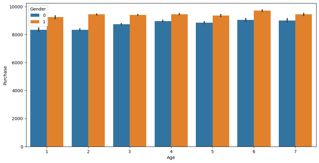
Conclusion 1
Across all ages, men spent more on the products.
# visualization by occupation
sns.barplot('Occupation', 'Purchase', hue='Gender', data=df)
/Users/pranav/mambaforge/lib/python3.10/site-packages/seaborn/_decorators.py:36: FutureWarning: Pass the following variables as keyword args: x, y. From version 0.12, the only valid positional argument will be `data`, and passing other arguments without an explicit keyword will result in an error or misinterpretation.
warnings.warn(
<Axes: xlabel='Occupation', ylabel='Purchase'>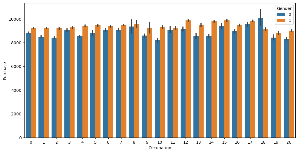
Conclusion 2
Only women in Occupation 18 spent more than men in the same occupation. We can conclude that men spent more irrespective of the occupation.
# visualization by product category
sns.barplot('Product_Category_1', 'Purchase', hue='Gender', data=df)
/Users/pranav/mambaforge/lib/python3.10/site-packages/seaborn/_decorators.py:36: FutureWarning: Pass the following variables as keyword args: x, y. From version 0.12, the only valid positional argument will be `data`, and passing other arguments without an explicit keyword will result in an error or misinterpretation.
warnings.warn(
<Axes: xlabel='Product_Category_1', ylabel='Purchase'>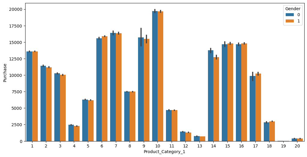
# visualization by product category
sns.barplot('Product_Category_2', 'Purchase', hue='Gender', data=df)
/Users/pranav/mambaforge/lib/python3.10/site-packages/seaborn/_decorators.py:36: FutureWarning: Pass the following variables as keyword args: x, y. From version 0.12, the only valid positional argument will be `data`, and passing other arguments without an explicit keyword will result in an error or misinterpretation.
warnings.warn(
<Axes: xlabel='Product_Category_2', ylabel='Purchase'>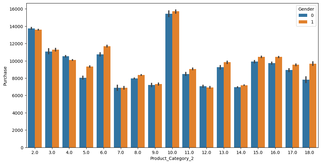
# visualization by product category
sns.barplot('Product_Category_3', 'Purchase', hue='Gender', data=df)
/Users/pranav/mambaforge/lib/python3.10/site-packages/seaborn/_decorators.py:36: FutureWarning: Pass the following variables as keyword args: x, y. From version 0.12, the only valid positional argument will be `data`, and passing other arguments without an explicit keyword will result in an error or misinterpretation.
warnings.warn(
<Axes: xlabel='Product_Category_3', ylabel='Purchase'>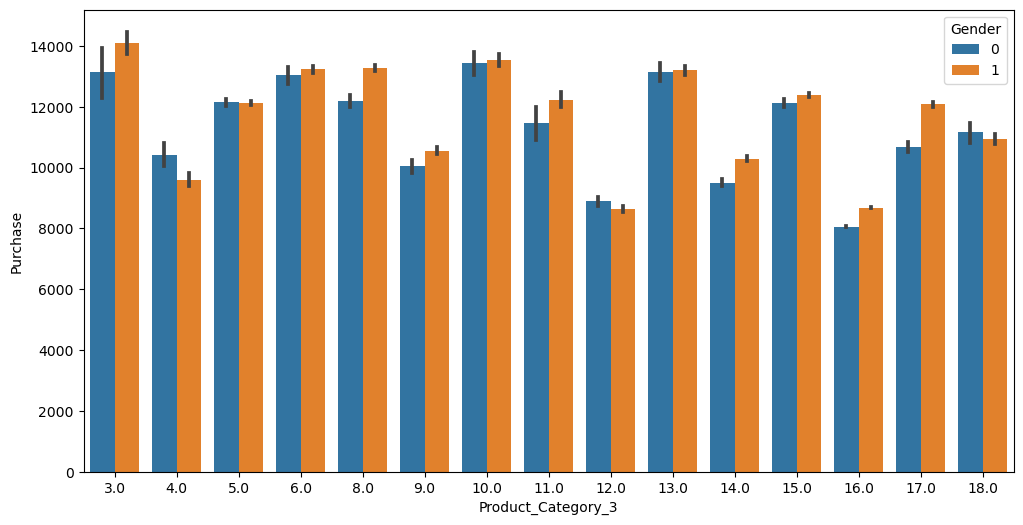
Conclusion 3
That’s interesting. Even though Product Category 1 has the most expensive product (Product 10 costs $20,000), a lot of the other products in the category have not been bought. This is probably why there is such a negative correlation in the overall purchase amount with this product category. Also, the purchasing behaviour based on gender is almost equal in this product category, which can’t be said for the other product categories.
Splitting the dataset
Now that we are done with our feature scaling and analysis, let’s split the dataset again.
df_test = df[df['Purchase'].isnull()]
df_train = df[~df['Purchase'].isnull()]
Train/Test Split
X = df_train.drop('Purchase',axis=1)
X.head(2)| Gender | Age | Occupation | Stay_In_Current_City_Years | Marital_Status | Product_Category_1 | Product_Category_2 | Product_Category_3 | B | C | |
|---|---|---|---|---|---|---|---|---|---|---|
| 0 | 0 | 1 | 10 | 2 | 0 | 3 | 8.0 | 16.0 | 0 | 0 |
| 1 | 0 | 1 | 10 | 2 | 0 | 1 | 6.0 | 14.0 | 0 | 0 |
y = df_train['Purchase']
y.head(2)
0 8370.0
1 15200.0
Name: Purchase, dtype: float64print(X.shape)
print(y.shape)(550068, 10)
(550068,)from sklearn.model_selection import train_test_split
X_train, X_test, y_train, y_test = train_test_split(
X, y, test_size=0.33, random_state=42)Feature Scaling
from sklearn.preprocessing import StandardScaler
sc = StandardScaler()
X_train = sc.fit_transform(X_train)
X_test = sc.transform(X_test)
The data is now ready for modeling.