pranav_shirole - Predicting the sale price of bulldozers sold at auctions

In this blog post, we will be predicting the sale price of bulldozers sold at auctions, based on the usage, equipment type, and configuration. The data is sourced from auction result postings and includes information on usage and equipment configurations.

The data for this competition on Kaggle is split into three parts:
- train.csv is the training set, which contains data through the end of 2011. - valid.csv is the validation set, which contains data from January 1, 2012 - April 30, 2012. - test.csv is the test set, which contains data from May 1, 2012 - Novemeber 2012.

The key fields in train.csv are: - SalesID: the unique identifier of the sale - MachineID: the unique identifier of a machine. A machine can be sold multiple times. - saleprice: what the machine sold for at auction - saledata: the date of the sale

import fastbook
fastbook.setup_book()

Let’s download the necessary libraries we’ll require throughout the notebook.

from fastbook import *
from kaggle import api
from pandas.api.types import is_string_dtype, is_numeric_dtype, is_categorical_dtype
from fastai.tabular.all import *
from sklearn.ensemble import RandomForestRegressor
from sklearn.tree import DecisionTreeRegressor
from dtreeviz.trees import *
from IPython.display import Image, display_svg, SVG

pd.options.display.max_rows = 20
pd.options.display.max_columns = 8

We’ll download the data from Kaggle using the Kaggle API.

creds = '{"username":"xxxx","key":"xxxx"}'

cred_path = Path('~/.kaggle/kaggle.json').expanduser()
if not cred_path.exists():
    cred_path.parent.mkdir(exist_ok=True)
    cred_path.write_text(creds)
    cred_path.chmod(0o600)

Let’s pick a path to download the dataset to.

path = URLs.path('bluebook')
path

Path('/home/pranav/.fastai/archive/bluebook')

We’ll use the Kaggle API to download the dataset to that path and extract it.

if not path.exists():
    path.mkdir()
    api.competition_download_cli('bluebook-for-bulldozers', path=path)
    file_extract(path)

Path.BASE_PATH = path
path.ls(file_type='text')

(#7) [Path('TrainAndValid.csv'),Path('Valid.csv'),Path('random_forest_benchmark_test.csv'),Path('Test.csv'),Path('median_benchmark.csv'),Path('ValidSolution.csv'),Path('Machine_Appendix.csv')]

The Dataset

No that we have downloaded our dataset, let’s take a look at it. We’ll read the training set into a Pandas dataframe. We’ll specify low_memory=False unless Pandas runs out of memory and returns an error. The low_memory parameter, which is True by default, tells Pandas to look at only a few rows of data at a time to figure out what type of data is in each column.

df = pd.read_csv(path/'TrainAndValid.csv', low_memory=False)

df.head()

	SalesID	SalePrice	MachineID	ModelID	...	Blade_Type	Travel_Controls	Differential_Type	Steering_Controls
0	1139246	66000.0	999089	3157	...	NaN	NaN	Standard	Conventional
1	1139248	57000.0	117657	77	...	NaN	NaN	Standard	Conventional
2	1139249	10000.0	434808	7009	...	NaN	NaN	NaN	NaN
3	1139251	38500.0	1026470	332	...	NaN	NaN	NaN	NaN
4	1139253	11000.0	1057373	17311	...	NaN	NaN	NaN	NaN

5 rows × 53 columns

df.shape

(412698, 53)

The dataset contains 412,698 rows of data and 53 columns. That’s a lot of data for us to look at!

df.columns

Index(['SalesID', 'SalePrice', 'MachineID', 'ModelID', 'datasource',
       'auctioneerID', 'YearMade', 'MachineHoursCurrentMeter', 'UsageBand',
       'saledate', 'fiModelDesc', 'fiBaseModel', 'fiSecondaryDesc',
       'fiModelSeries', 'fiModelDescriptor', 'ProductSize',
       'fiProductClassDesc', 'state', 'ProductGroup', 'ProductGroupDesc',
       'Drive_System', 'Enclosure', 'Forks', 'Pad_Type', 'Ride_Control',
       'Stick', 'Transmission', 'Turbocharged', 'Blade_Extension',
       'Blade_Width', 'Enclosure_Type', 'Engine_Horsepower', 'Hydraulics',
       'Pushblock', 'Ripper', 'Scarifier', 'Tip_Control', 'Tire_Size',
       'Coupler', 'Coupler_System', 'Grouser_Tracks', 'Hydraulics_Flow',
       'Track_Type', 'Undercarriage_Pad_Width', 'Stick_Length', 'Thumb',
       'Pattern_Changer', 'Grouser_Type', 'Backhoe_Mounting', 'Blade_Type',
       'Travel_Controls', 'Differential_Type', 'Steering_Controls'],
      dtype='object')

Looking at the data, we can try to gauge what kind of information is in each column.
Let’s have a look at the ordinal columns, i.e. columns containing strings or similar but where those strings have a natural ordering. ProductSize seems like it could be one of those columns.

df['ProductSize'].unique()

array([nan, 'Medium', 'Small', 'Large / Medium', 'Mini', 'Large', 'Compact'], dtype=object)

We can tell Pandas about a suitable ordering of these levels.

sizes = 'Large', 'Large / Medium', 'Medium', 'Small', 'Mini', 'Compact'

df['ProductSize'] = df['ProductSize'].astype('category')
df['ProductSize'].cat.set_categories(sizes, ordered=True, inplace=True)

The metric we’ll be using is the root mean squared log error (RMLSE) between the actual and predicted prices, since that is what Kaggle suggests for this dataset. We need to take the log of the prices, so that the m_rmse of that value will give us what we ultimately need.

dep_var = 'SalePrice'
df[dep_var] = np.log(df[dep_var])

Data Preprocessing

Handling Dates

Our model should know more than whether a date is more recent or less recent than another. We might want our model to make decisions based on that date’s day of the week, on whether a day is a holiday, on what month it is in, and so forth. To do this, we’ll replace every data column with a set of date metadata columns, such as holiday, day of week, and month. These columns provide categorical data that might be useful.
fastai comes with a function add_datepart that will do this for us when we pass a column name that contains dates.

df = add_datepart(df, 'saledate')

Let’s do the same for our test set.

df_test = pd.read_csv(path/'Test.csv', low_memory=False)
df_test = add_datepart(df_test, 'saledate')

df.shape

(412698, 65)

We can see that instead of the original 53, we now have 65 columns in our dataset. Let’s see what the new columns are.

' '.join(o for o in df.columns if o.startswith('sale'))

'saleYear saleMonth saleWeek saleDay saleDayofweek saleDayofyear saleIs_month_end saleIs_month_start saleIs_quarter_end saleIs_quarter_start saleIs_year_end saleIs_year_start saleElapsed'

Handling Strings and Missing Data

fastai’s class TabularPandas wraps a Pandas dataframe and provides a few conveniences. To populate a TabularPandas, we will use two TabularProcs - Categorify and FillMissing.
A TabularProc is like a regular Transform, except: - it returns the exact same object that’s passed to it, after modifying the object in place. - it runs the transform once, when the data is first passed in, rather than as the data is accessed.

Categorify is a TabularProc that replaces a categorical column with a numeric column. FillMissing is a TabularProc that replaces missing values with the median of the column, and creates a new Boolean column that is set to True for any row where the value was missing.

procs = [Categorify, FillMissing]

TabularPandas will also handle splitting the dataset into training and validation sets for us. But we’ll want to define our validation data so that it has the same sort of relationship to the training data as the test set will have. As mentioned in the data description above, the test set covers a six-month period from May 2012, which is later in time than any date in the training set. It means that if we’re going to have a useful validation set, we’ll want it to tbe later in time than the training set. The Kaggle training data ends in April 2012, so we will define a narrower training set that consists only of the training data from before November 2011, and we’ll define a validation set consisting of data from after 2011.
To do this we use np.where, which will return (as the first element of a tuple) the indices of all True values.

cond = (df.saleYear < 2011) | (df.saleMonth < 10)
train_idx = np.where(cond)[0]
valid_idx = np.where(~cond)[0]
splits = (list(train_idx), list(valid_idx))

TabularPandas needs to be told which columns are continuous and which are categorical. We can handle that automatically using the helper function cont_cat_split.

cont, cat = cont_cat_split(df, 1, dep_var=dep_var)

to = TabularPandas(df, procs, cat, cont, y_names=dep_var, splits=splits)

TabularPandas provides train and valid attributes.

len(to.train), len(to.valid)

(404710, 7988)

to.show(5)

	UsageBand	fiModelDesc	fiBaseModel	fiSecondaryDesc	fiModelSeries	fiModelDescriptor	ProductSize	fiProductClassDesc	state	ProductGroup	ProductGroupDesc	Drive_System	Enclosure	Forks	Pad_Type	Ride_Control	Stick	Transmission	Turbocharged	Blade_Extension	Blade_Width	Enclosure_Type	Engine_Horsepower	Hydraulics	Pushblock	Ripper	Scarifier	Tip_Control	Tire_Size	Coupler	Coupler_System	Grouser_Tracks	Hydraulics_Flow	Track_Type	Undercarriage_Pad_Width	Stick_Length	Thumb	Pattern_Changer	Grouser_Type	Backhoe_Mounting	Blade_Type	Travel_Controls	Differential_Type	Steering_Controls	saleIs_month_end	saleIs_month_start	saleIs_quarter_end	saleIs_quarter_start	saleIs_year_end	saleIs_year_start	auctioneerID_na	MachineHoursCurrentMeter_na	SalesID	MachineID	ModelID	datasource	auctioneerID	YearMade	MachineHoursCurrentMeter	saleYear	saleMonth	saleWeek	saleDay	saleDayofweek	saleDayofyear	saleElapsed	SalePrice
0	Low	521D	521	D	#na#	#na#	#na#	Wheel Loader - 110.0 to 120.0 Horsepower	Alabama	WL	Wheel Loader	#na#	EROPS w AC	None or Unspecified	#na#	None or Unspecified	#na#	#na#	#na#	#na#	#na#	#na#	#na#	2 Valve	#na#	#na#	#na#	#na#	None or Unspecified	None or Unspecified	#na#	#na#	#na#	#na#	#na#	#na#	#na#	#na#	#na#	#na#	#na#	#na#	Standard	Conventional	False	False	False	False	False	False	False	False	1139246	999089	3157	121	3.0	2004	68.0	2006	11	46	16	3	320	1.163635e+09	11.097410
1	Low	950FII	950	F	II	#na#	Medium	Wheel Loader - 150.0 to 175.0 Horsepower	North Carolina	WL	Wheel Loader	#na#	EROPS w AC	None or Unspecified	#na#	None or Unspecified	#na#	#na#	#na#	#na#	#na#	#na#	#na#	2 Valve	#na#	#na#	#na#	#na#	23.5	None or Unspecified	#na#	#na#	#na#	#na#	#na#	#na#	#na#	#na#	#na#	#na#	#na#	#na#	Standard	Conventional	False	False	False	False	False	False	False	False	1139248	117657	77	121	3.0	1996	4640.0	2004	3	13	26	4	86	1.080259e+09	10.950807
2	High	226	226	#na#	#na#	#na#	#na#	Skid Steer Loader - 1351.0 to 1601.0 Lb Operating Capacity	New York	SSL	Skid Steer Loaders	#na#	OROPS	None or Unspecified	#na#	#na#	#na#	#na#	#na#	#na#	#na#	#na#	#na#	Auxiliary	#na#	#na#	#na#	#na#	#na#	None or Unspecified	None or Unspecified	None or Unspecified	Standard	#na#	#na#	#na#	#na#	#na#	#na#	#na#	#na#	#na#	#na#	#na#	False	False	False	False	False	False	False	False	1139249	434808	7009	121	3.0	2001	2838.0	2004	2	9	26	3	57	1.077754e+09	9.210340
3	High	PC120-6E	PC120	#na#	-6E	#na#	Small	Hydraulic Excavator, Track - 12.0 to 14.0 Metric Tons	Texas	TEX	Track Excavators	#na#	EROPS w AC	#na#	#na#	#na#	#na#	#na#	#na#	#na#	#na#	#na#	#na#	2 Valve	#na#	#na#	#na#	#na#	#na#	None or Unspecified	#na#	#na#	#na#	#na#	#na#	#na#	#na#	#na#	#na#	#na#	#na#	#na#	#na#	#na#	False	False	False	False	False	False	False	False	1139251	1026470	332	121	3.0	2001	3486.0	2011	5	20	19	3	139	1.305763e+09	10.558414
4	Medium	S175	S175	#na#	#na#	#na#	#na#	Skid Steer Loader - 1601.0 to 1751.0 Lb Operating Capacity	New York	SSL	Skid Steer Loaders	#na#	EROPS	None or Unspecified	#na#	#na#	#na#	#na#	#na#	#na#	#na#	#na#	#na#	Auxiliary	#na#	#na#	#na#	#na#	#na#	None or Unspecified	None or Unspecified	None or Unspecified	Standard	#na#	#na#	#na#	#na#	#na#	#na#	#na#	#na#	#na#	#na#	#na#	False	False	False	False	False	False	False	False	1139253	1057373	17311	121	3.0	2007	722.0	2009	7	30	23	3	204	1.248307e+09	9.305651

We can see that the data is still displayed as strings for categories.
However, the underlying items are all numeric.

to.items.head(5)

	SalesID	SalePrice	MachineID	ModelID	...	saleIs_year_start	saleElapsed	auctioneerID_na	MachineHoursCurrentMeter_na
0	1139246	11.097410	999089	3157	...	1	1.163635e+09	1	1
1	1139248	10.950807	117657	77	...	1	1.080259e+09	1	1
2	1139249	9.210340	434808	7009	...	1	1.077754e+09	1	1
3	1139251	10.558414	1026470	332	...	1	1.305763e+09	1	1
4	1139253	9.305651	1057373	17311	...	1	1.248307e+09	1	1

5 rows × 67 columns

The conversion of categorical columns to numbers is done by simply replacing each unique level with a number. The numbers associated with the levels are chosen consecutively as they are seen in a column, so there’s no particular meaning to the numbers in categorical columns after conversion. The exception is if you first convert a column to a Pandas ordered category (ProductSize), in which case the ordering you chose is used.
We can see the mapping by looking at the classes attribute.

to.classes['ProductSize']

['#na#', 'Large', 'Large / Medium', 'Medium', 'Small', 'Mini', 'Compact']

Now that we are done with the preprocessing stage, let’s save our data.

save_pickle(path/'to.pkl', to)

Model Training

Now that our data is all numeric, and there are no missing values, we can train our model.
Let’s define our independent and dependent variables.

xs, y = to.train.xs, to.train.y
valid_xs, valid_y = to.valid.xs, to.valid.y

Decision Trees

Let us create a Decision Tree.

m = DecisionTreeRegressor(max_leaf_nodes = 4)
m.fit(xs, y)

DecisionTreeRegressor(max_leaf_nodes=4)

Let’s create a simple model first with only four leaf nodes.
We can display the tree to see what it’s learned.

draw_tree(m, xs, size=7, leaves_parallel=True, precision=2)

svg

We can also show the information using the dtreeviz library.

samp_idx = np.random.permutation(len(y))[:500]
dtreeviz(m, xs.iloc[samp_idx], y.iloc[samp_idx], xs.columns, dep_var, 
        fontname='DejaVu Sans', scale=1.6, label_fontsize=10, orientation='LR')

svg

This shows a chart of the distribution of the data for each split point. Here we see one of the benefits of creating a simple model first. We can clearaly see that there’s a problem with our YearMade data, which shows that there are bulldozers made in the year 1000. This is probably just a missing value code (a value that doesn’t otherwise appear in the data and that is used as a placeholder in cases where a value is missing). For modeling purposes, 100 is fine, but this outlier makes visualizing the values we are interested in more difficult. So we’ll replace it with 1950.

xs.loc[xs['YearMade'] < 1900, 'YearMade'] = 1950
valid_xs.loc[valid_xs['YearMade'] < 1900, 'YearMade'] = 1950

Even though it doesn;t change the result of the model in any significant way, that change makes the split much clearer in the tree visualization.

m = DecisionTreeRegressor(max_leaf_nodes = 4).fit(xs, y)
dtreeviz(m, xs.iloc[samp_idx], y.iloc[samp_idx], xs.columns, dep_var, 
        fontname='DejaVu Sans', scale=1.6, label_fontsize=10, orientation='LR')

svg

Now let’s have the decision tree algorithm build a bigger tree. We’ll not pass in any stopping criteria.

m = DecisionTreeRegressor()
m.fit(xs, y)

DecisionTreeRegressor()

We’ll create a little function to check the root mean squared error of our model (m_rmse) of our model.

def r_mse(pred, y):
    return round(math.sqrt(((pred-y)**2).mean()), 6)

def m_rmse(m, xs, y):
    return r_mse(m.predict(xs), y)

m_rmse(m, xs, y)

0.0

Hmm, here our model is showing an error of 0. But that doesn’t mean our model is perfect. It probably means that our model is badly overfitting. Let’s check the error on the validation set.

m_rmse(m, valid_xs, valid_y)

0.334935

Here’s why we’re overfitting so badly.

# no. of leaf nodes, no. of datapoints
m.get_n_leaves(), len(xs)

(324560, 404710)

We’ve got nearly as many leaf nodes as data points! That’s a little too much. sklearn’s default settings allow it to continue splitting nodes until there is only one item in each leaf node. Let’s change the stopping rule.

m = DecisionTreeRegressor(min_samples_leaf=25)
m.fit(to.train.xs, to.train.y)
m_rmse(m, xs, y), m_rmse(m, valid_xs, valid_y)

(0.248593, 0.323339)

That looks much better. Let’s check the number of leaves again.

m.get_n_leaves()

Random Forests

A random forest is a model that averages the predictions of a large number of decision trees, which are generated by randomly varying various parameters that specify what data is used to train the tree and other tree parameters.
We create a random forest just like we create a decision tree, except now, we’re alsp specifying the paramters that indicate how many trees should be in the forest, how we should subset the data items (the rows), and how we should subset the fields (the columns).

def rf(xs, y, n_estimators=100, max_samples=200_000,
      max_features=0.5, min_samples_leaf=5, **kwargs):
    return RandomForestRegressor(n_jobs=-1, n_estimators=n_estimators,
                                    max_samples=max_samples, max_features=max_features,
                                    min_samples_leaf=min_samples_leaf, oob_score=True).fit(xs, y)

m = rf(xs, y)

m_rmse(m, xs, y), m_rmse(m, valid_xs, valid_y)

(0.169731, 0.232174)

Our validation RMSE is much improved compared to the one produced by the one decision tree.
To see the impact of n_estimators, let’s get the predictions from each individual tree in our forest (these are in the estimators_ attribute).

preds = np.stack([t.predict(valid_xs) for t in m.estimators_])

r_mse(preds.mean(0), valid_y)

0.232174

As you can see, preds.mean(0) gives the same results as our random forest.
Let’s see what happens to the RMSE as we add more and more trees.

plt.plot([r_mse(preds[:i+1].mean(0), valid_y) for i in range(100)])

[<matplotlib.lines.Line2D at 0x7f039ea0bf10>]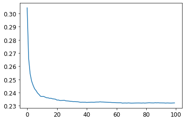

As you can see, the improvement levels off quite a bit after around 30 trees.

The performance on our validation set is worse than on our training set. Random forests have out-of-bad (OOB) error that can help us with this.

Model Interpretation

Out-of-Bag Error

In a random forest, each tree is trained on a different subset of the training data. The OOB error is a way of measuring prediction error on the training set by only including in the calculation of a row’s error trees where that row was not included in training. This allows us to see whether the model is overfitting, without needing a separate validation set. This is particularly beneficial in cases where we have only a small amount of training data, as it allows us to see whether our model generalizes without removing items to create a validation set. The OOB predictions are available in the oob_prediction_ attribute. We compare them to the training labels, since this is being calculated on trees using the training set.

r_mse(m.oob_prediction_, y)

0.208747

We can see that our OOB error is much lower than our validation set error. This means that something else is causing that error, in addition to normal generalization error.

Tree Variance for Prediction Confidence

How confident are we in our predictions using a particular row of data?
We saw how the model averages the individual tree’s predictions to get an overall prediction, i.e. an estimate of the value. But how can we know the confidence of the estimate? One simple way is to use the standard deviation of predictions across the trees, instead of just the mean. This tells us the relative confidence of the predictions. In general, we would want to be more cautious of using the results for rows where trees give very different results (higher standard deviations), compared to cases where they are more consistence (lower standard deviations).

preds = np.stack([t.predict(valid_xs) for t in m.estimators_])

preds.shape

(100, 7988)

Now we have a prediction for every tree and every auction (100 trees and 7,988 auctions) in the validation set. Using this, we can get the standard deviation of the predictions over all the trees, for every auction.

preds_std = preds.std(0)

Let’s find the standard deviations for the predictions for the first five auctions, i.e. the first five rows of the validation set.

preds_std[:5]

array([0.253279  , 0.10988732, 0.10787489, 0.25965299, 0.12552832])

As you can see, the confidence in the predictions varies widely. For some auctions, there is a low standard deviation because the trees agree. For others, it’s higher, as the trees don’t agree. If you were using this model to decide what items to bid on at auction, a low-confidence prediction might cause you to look more carefully at an item before you made a bid.

Feature Importance

Which columns are the strongest predictors?
Feature Importance gives us insight into how a model is making predictions. We can use the feature_importances_ attribute. Let’s create a function to pop them into a dataframe and sort them.

def rf_feat_importance(m, df):
    return pd.DataFrame({'cols': df.columns, 'imp': m.feature_importances_}
                       ).sort_values('imp', ascending=False)

fi = rf_feat_importance(m, xs)
fi[:10]

	cols	imp
57	YearMade	0.176429
6	ProductSize	0.119205
30	Coupler_System	0.117753
7	fiProductClassDesc	0.072875
54	ModelID	0.054168
65	saleElapsed	0.049664
31	Grouser_Tracks	0.048707
3	fiSecondaryDesc	0.045853
12	Enclosure	0.034020
1	fiModelDesc	0.033681

The feature importances of our model show that the first few most importance columns have much higher importance scores than the rest, with YearMade and ProductSize being at the top of the list.
A plot of the feature importances shows the relative importance more clearly.

def plot_fi(fi):
    return fi.plot('cols', 'imp', 'barh', figsize=(12,7), legend=False)

plot_fi(fi[:30])

<AxesSubplot:ylabel='cols'>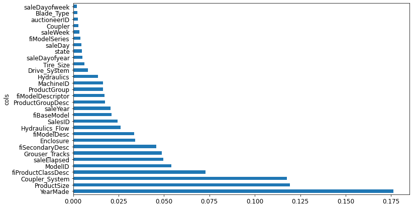

Removing Low-Importance Variables

Which columns can we ignore?
We could just use a subset of the columns by removing the variables of low importance and still get good results. Let’s try just keeping those with a feature importance greater than 0.005.

to_keep = fi[fi.imp > 0.005].cols
len(to_keep)

We can retrain our model using just this subset of the columns.

xs_imp = xs[to_keep]
valid_xs_imp = valid_xs[to_keep]

m = rf(xs_imp, y)

And here’s the result:

m_rmse(m, xs_imp, y), m_rmse(m, valid_xs_imp, valid_y)

(0.180239, 0.230229)

Our validation accuracy is about the same but we have far fewer columns to study.

len(xs.columns), len(xs_imp.columns)

(66, 21)

Let’s look at our feature importance plot again.

plot_fi(rf_feat_importance(m, xs_imp))

<AxesSubplot:ylabel='cols'>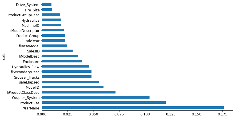

Removing Redundant Features

Which columns are effectively redundant with each other, for purposes of prediction?
There seem to be variables with similar meanings, for e.g. ProductGroup and ProductGroupDesc. Let’s try to remove any redundant features.

cluster_columns(xs_imp)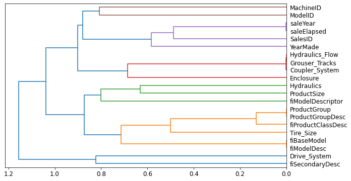

In this chart, the pairs of columns that are most similar are the ones that were merged together early. Unsurprisingly, the fields ProductGroup and ProductGroupDesc were merged quite early, along with saleYear and saleElapsed, and fiBaseModel and fiModelDesc. Let’s try removing some of these closely related features to see if the model can be simplified without impacting the accuracy.
First, we create a function that quickly trains a random forest and returns the OOB score, by using a lower max_samples and higher min_samples_leaf. The OOB score is a number returned by sklearn that ranges between 1.0 for a perfect model and 0.0 for a random model. We don’t need it to be very accurate; we’re just going to use t to compare different models, based on removing some of the possibly redundant columns.

def get_oob(df):
    m = RandomForestRegressor(n_estimators=40, min_samples_leaf=15,
                             max_samples=50000, max_features=0.5,
                             n_jobs=-1, oob_score=True)
    m.fit(df, y)
    return m.oob_score_

Here’s our baseline:

get_oob(xs_imp)

0.8773453848775988

Now we’ll try removing each of our potentially redundant variables, one at a time.

{c:get_oob(xs_imp.drop(c, axis=1)) for c in (
    'saleYear', 'saleElapsed', 
    'ProductGroupDesc', 'ProductGroup',
    'fiModelDesc', 'fiBaseModel', 
    'Hydraulics_Flow', 'Grouser_Tracks', 'Coupler_System')}

{'saleYear': 0.8768014266597242,
 'saleElapsed': 0.8719167973771567,
 'ProductGroupDesc': 0.8770285539401924,
 'ProductGroup': 0.8780539740440588,
 'fiModelDesc': 0.8753778428292395,
 'fiBaseModel': 0.8762011220745426,
 'Hydraulics_Flow': 0.8773475825106756,
 'Grouser_Tracks': 0.8776377009405991,
 'Coupler_System': 0.8771692298411222}

Now let’s try dropping multiple variables. We’ll drop one from each of the tightly aligned pairs we noticed earlier.

# maybe drop columns with higher oob score
to_drop = ['saleYear', 'ProductGroupDesc', 'fiBaseModel', 'Grouser_Tracks']
get_oob(xs_imp.drop(to_drop, axis=1))

0.8743584495396625

This is not much worse than the model with all the fields.
Let’s create dataframes without these columns.

xs_final = xs_imp.drop(to_drop, axis=1)
valid_xs_final = valid_xs_imp.drop(to_drop, axis=1)

Let’s save the dataframes.

save_pickle(path/'xs_final.pkl', xs_final)
save_pickle(path/'valid_xs_final.pkl', valid_xs_final)

Now we can check our RMSE again to confirm that the accuracy hasn’t changed substantially.

m = rf(xs_final, y)
m_rmse(m, xs_final, y), m_rmse(m, valid_xs_final, valid_y)

(0.18224, 0.231327)

By focusing on the most important variables, and removing some redundant ones, we’ve greatly simplified our model. Now, let’s see how those variables affect our predictions using partial dependence plots.

Partial Dependence

How do predictions vary, as we vary the columns?
As we’ve seen, the two most important predictors are ProductSize and YearMade. We’d like to understand the relationship between these predictors and sale price. It’s a good idea to first check the count of values per category to see how common each category is. For this, we’ll use the Pandas value_counts method.

p = valid_xs_final['ProductSize'].value_counts(sort=False).plot.barh()
c = to.classes['ProductSize']
plt.yticks(range(len(c)), c)

([<matplotlib.axis.YTick at 0x7f039c4c7220>,
  <matplotlib.axis.YTick at 0x7f039c4c75b0>,
  <matplotlib.axis.YTick at 0x7f039c4f18e0>,
  <matplotlib.axis.YTick at 0x7f039de4e100>,
  <matplotlib.axis.YTick at 0x7f039de4e610>,
  <matplotlib.axis.YTick at 0x7f039de4eb20>,
  <matplotlib.axis.YTick at 0x7f039de53070>],
 [Text(0, 0, '#na#'),
  Text(0, 1, 'Large'),
  Text(0, 2, 'Large / Medium'),
  Text(0, 3, 'Medium'),
  Text(0, 4, 'Small'),
  Text(0, 5, 'Mini'),
  Text(0, 6, 'Compact')])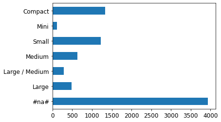

The largest group is #na#, which is the label fastai applies to missing values.
Let’s do the same thing for YearMade. Since this is a numeric feature, we’ll need to draw a histogram, which groups the year values into a few discrete bins.

ax = valid_xs_final['YearMade'].hist()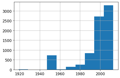

Other than the special value 1950, which we used for coding missing values, most of the data is from after 1990.

Partial dependence plots try to answer the question: if a row is varied on nothing other than the feature in question, how would it impact the dependent variable? For e.g., how does YearMade impact sale price, all other things being equal?
We’ll replace every single value in the YearMade column with 1950, and then calculate the predicted sale price for every auction, and take the average over all the auctions. Then we do the same for 1951, 1952, and so forth until 2011. This isolates the effect of only YearMade. With these averages, we can then plot each of these years on the x-axis, and each of the prediction on the y-axis. That gives us a partial dependence plot.

from sklearn.inspection import plot_partial_dependence

fig, ax = plt.subplots(figsize=(12,4))
plot_partial_dependence(m, valid_xs_final, ['YearMade', 'ProductSize'],
                       grid_resolution=20, ax=ax)

<sklearn.inspection._plot.partial_dependence.PartialDependenceDisplay at 0x7f039c5286d0>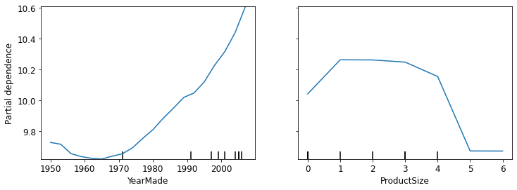

In the YearMade plot, we can clearly see a nearly linear relationship between year and price. Our dependent variable is after taking the logarithm, which means that in practice there is an exponential increase in price. Since depreciation is generally recognized as being a multiplicative factor over time, for a given sale date, varying year made ought to show an exponential relationship with sale price.
In the ProductSize plot, it shows that the final group, which is for missing values, has the lowest price. This is concerning and we would want to find out why it’s missing so often, and what that means. Missing values could sometimes be useful predictors, or sometimes they can indicate data leakage.

Tree Interpreter

For predicting with a particular row of data, what were the most important factors, and how did they influence the prediction?
Tree Interpreters help you identify which factors influence specific predictions.

import warnings
warnings.simplefilter('ignore', FutureWarning)

from treeinterpreter import treeinterpreter
from waterfall_chart import plot as waterfall

Let’s say we’re looking at some particular item in the auction. Our model might predict that this item will be very expensive, and we want to know why. So, we take that one row of data and put it throguh the first decision tree, looking to see what split is used at each point throughout the tree. For each split, we see what the increase or decrease in the addition is, compared to the parent node of the tree. We do this for every tree, and add up the total change in importance by split variable.
For instance, let’s pick the first few rows of our validation set.

row = valid_xs_final.iloc[:5]

We can pass these to treeinterpreter.

prediction, bias, contributions = treeinterpreter.predict(m, row.values)

prediction is the prediction that the random forest makes. bias is the prediction based on taking the mean of the dependent variable (i.e. the model that is the root of every tree). contributions tell us the total change in prediction due to each of the independent variables. So, the sum of contributions and bias must include predictions, for each row.
Let’s look at just the first row.

prediction[0], bias[0], contributions[0].sum()

(array([10.02467957]), 10.104720584542706, -0.0800410097588184)

The clearest way to display the contributions is with a waterfall plot.

waterfall(valid_xs_final.columns, contributions[0], threshold=0.08, 
          rotation_value=45,formatting='{:,.3f}');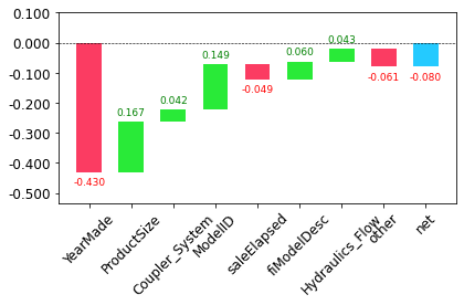

This shows how the positive and negative contributions from all the independent variables sum up to create the final prediction, which is the right-hand column labeled “net”.
This kind of information is most useful in production since you can use it to provide useful information to users of your data product about the underlying reasoning behind the predictions.

Extrapolation Problem

A random forest just averages the predictions of a number of trees. And a tree simply predicts the average value of the rows in a leaf. Thus, a tree and a random forest can never predict values outside of the range of the training data. This is particularly problematic for data where there is a trend over time, such as inflation, and you wish to make predictions for a future time. Your predictions will be systematically too low. Moreover, random forests are not able to extrapolate outside of the types of data they have seen, in a more general sense. That’s why we need to make sure that our validation set does not contain out-of-domain data.

Finding Out-Of-Domain Data

We’ll try to predict whether a row is in the validation set or training set. For this, we’ll combine our training and validation sets together, create a dependent variable that represents which dataset each row comes from, build a random forest using that data, and get its feature importance.

df_dom = pd.concat([xs_final, valid_xs_final])
is_valid = np.array([0]*len(xs_final) + [1]*len(valid_xs_final))

m = rf(df_dom, is_valid)
rf_feat_importance(m, df_dom)[:6]

	cols	imp
5	saleElapsed	0.896474
10	SalesID	0.078574
13	MachineID	0.019742
0	YearMade	0.001183
4	ModelID	0.000789
16	Tire_Size	0.000525

This shows that there are three columns that differ significantly between the training and validation sets: saleElapsed, SalesID, and MachineID.
saleElapsed: it’s the number of days between the start of the dataset and each row, so it directly encodes the date.
SalesID: the identifiers for auction sales might increment over time.
MachineID: the same might be happening for individual items sold in the auctions.

Let’s get a baseline of the original random forest model’s RMSE, then see what the effect is of removing each of these columns in turn.

m = rf(xs_final, y)
print('orig', m_rmse(m, valid_xs_final, valid_y))

for c in ('SalesID', 'saleElapsed', 'MachineID'):
    m = rf(xs_final.drop(c, axis=1), y)
    print(c, m_rmse(m, valid_xs_final.drop(c, axis=1), valid_y))

orig 0.231707
SalesID 0.229693
saleElapsed 0.234533
MachineID 0.230408

It looks like we should be able to remove SalesID and MachineID without losing any accuracy. Let’s check.

time_vars = ['SalesID', 'MachineID']
xs_final_time = xs_final.drop(time_vars, axis=1)
valid_xs_time = valid_xs_final.drop(time_vars, axis=1)

m = rf(xs_final_time, y)
m_rmse(m, valid_xs_time, valid_y)

0.228485

Removing these variables has slightly improved the model’s accuracy; but more importantly, it should make it more resilient over time, and easier to maintain and understand.

One thing that might help in our case is to simply avoid using old data. Often, old data shows relationships that just aren’t valid any more. Let’s just try using the most recent few years of the data.

xs['saleYear'].hist()

<AxesSubplot:>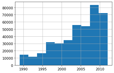

Let’s consider only the sales after the year 2004.

filt = xs['saleYear'] > 2004
xs_filt = xs_final_time[filt]
y_filt = y[filt]

Here’s the result of training on this subset.

m = rf(xs_filt, y_filt)
m_rmse(m, xs_filt, y_filt), m_rmse(m, valid_xs_time, valid_y)

(0.176994, 0.228504)

It’s a little better, which shows that you shouldn’t always just use your entire dataset; sometimes a subset can be better.

Using a Neural Network

We’ll now try using a neural network. We can use the same approach to build a neural network model. Let’s first replicate the steps we took to set up the TabularPandas object.

df_nn = pd.read_csv(path/'TrainAndValid.csv', low_memory=False)
df_nn['ProductSize'] = df_nn['ProductSize'].astype('category')
df_nn['ProductSize'].cat.set_categories(sizes, ordered=True, inplace=True)
df_nn[dep_var] = np.log(df_nn[dep_var])
df_nn = add_datepart(df_nn, 'saledate')

We can leverage the work we did to trim unwanted columns in the random forest by using the same set of columns for our neural network.

df_nn_final = df_nn[list(xs_final_time.columns) + [dep_var]]

Categorical columns are handled very differently in neural networks, compared to the decision tree approach. In a neural network, a great way to handle categorical variables is by using embeddings. To create embeddings, fastai needs to determine which columns should be treated as categorical variables. It does this by comparing the number of distinct levels in the variable to the value of the max_card parameter. If it’s lower, fastai will treat the variable as categorical. Embedding sizes larger than 10,000 should generally only be used after you’ve tested whether there are better ways to group the variable, so we’ll use 9,000 as our max_card.

cont_nn, cat_nn = cont_cat_split(df_nn_final, max_card=9000, dep_var=dep_var)

There is one variable that we absolutely do not want to treat as categorical: the saleElapsed variable. A categorical variable, by definition, cannot extrapolate outside the range of values that it has seen, but we want to be able to predict auction sales in the future.
Let’s verify that cont_cat_split did the correct thing.

cont_nn

['saleElapsed']

Let’s look at the cardinality of each of the categorical variables that we have chosen so far.

df_nn_final[cat_nn].nunique()

YearMade                73
ProductSize              6
Coupler_System           2
fiProductClassDesc      74
ModelID               5281
fiSecondaryDesc        177
Enclosure                6
fiModelDesc           5059
Hydraulics_Flow          3
fiModelDescriptor      140
ProductGroup             6
Hydraulics              12
Drive_System             4
Tire_Size               17
dtype: int64

The fact that there are two variables pertaining to the “model” of the equipment, both with similar high cardinalities, suggests that they may contain similar, redundant information. Note that we would not necessarily see this when analyzing redundant features, since that relies on similar variables being sorted in the same order, i.e. they need to have similarly named levels. Having a column with 5,000 levels means needing 5,000 columns in our embedding matrix, which would be nice to avoid if possible.
Let’s see what the impact of removing one of these model columns has on the random forest.

xs_filt2 = xs_filt.drop('fiModelDescriptor', axis=1)
valid_xs_time2 = valid_xs_time.drop('fiModelDescriptor', axis=1)
m2 = rf(xs_filt2, y_filt)
m_rmse(m2, xs_filt2, y_filt), m_rmse(m2, valid_xs_time2, valid_y)

(0.175986, 0.229453)

There’s minimal impact, so we will remove it as a perdictor for our neural network.

cat_nn.remove('fiModelDescriptor')

We can create our TabularPandas object in the same way as when we created our random forest, with one very important addition: normalization. A random forest does not need any normalization since the tree building procedure cares only about the order of values in a variable, not at all about how they are scaled. But a neural network does care about this and thus, we add the Normalize processor when we build our TabularPandas object.

procs_nn = [Categorify, FillMissing, Normalize]
to_nn = TabularPandas(df_nn_final, procs_nn, cat_nn, cont_nn,
                     splits=splits, y_names=dep_var)

Since tabular models and data don’t generally require much GPU RAM, we can use larger batch sizes.

dls = to_nn.dataloaders(1024)

It’s a good idea to set y_range for regression models, so let’s find out the min and max of our dependent variable.

y = to_nn.train.y
y.min(), y.max()

(8.465899, 11.863583)

We can now create the Learner to create this tabular model.
By default, for tabular data, fastai creates a neural network with two hidden layers, with 200 and 100 activations, respectively. This works well for small datasets, but here we’ve got quite a large dataset, so we increase the layer sizes to 500 and 250.

from fastai.tabular.all import *

---------------------------------------------------------------------------

ModuleNotFoundError                       Traceback (most recent call last)

Cell In[1], line 1
----> 1 from fastai.tabular.all import *


ModuleNotFoundError: No module named 'fastai'

learn = tabular_learner(dls, y_range=(8,12), layers=[500, 250],
                       n_out=1, loss_func=F.mse_loss)

learn.lr_find()

SuggestedLRs(lr_min=0.0033113110810518267, lr_steep=0.00015848931798245758)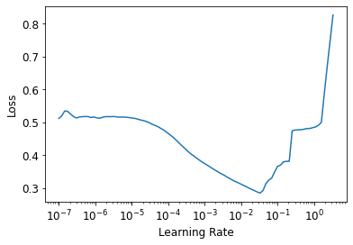

There’s no need to use fine_tune, so we’ll train with fit_one_cycle for a few epochs and see how it looks.

learn.fit_one_cycle(5, 3.3e-3)

epoch	train_loss	valid_loss	time
0	0.069181	0.062983	01:33
1	0.057557	0.062395	01:27
2	0.050993	0.056399	01:29
3	0.045013	0.051584	01:26
4	0.041281	0.051339	01:37

We can use our r_mse function to compare the result to the random forest result we got earlier.

preds, targs = learn.get_preds()
r_mse(preds, targs)

0.226582

It’s quite a bit better than the random forest, although it took longer to train.

Ensembling

Another thing that can help with generalization is to use several models and average their prediction - a technique known as ensembling.
We have trained two very different models, trained using very different algorithms: random forest, and a neural network. It would be reasonable to expect that the kinds of errors that each one makes would be quite different. Thus, we might expect that the average of their predictions would be better than either one’s individual predictions. We can create an ensemble of the random forest adn the neural network.
The PyTorch model and sklearn model create data of different types: PyTorch gives us a rank-2 tensor (i.e. a colun matrix), whereas NumPy gives us a rank-1 array (a vector). squeeze removes any unit axes from a tensor, and to_np converts it into a NumPy array.

rf_preds = m.predict(valid_xs_time)
ens_preds = (to_np(preds.squeeze()) + rf_preds) / 2

r_mse(ens_preds, valid_y)

0.222424

This is a much better result. In fact, this result is better than any score shown on the Kaggle leaderboard. However, it isn’t directly comparable since the leaderboard uses a separate test dataset that we do not have access to. But our results are certainly encouraging!