Analyzing China’s GDP growth

In this blog post, we will analyze China’s GDP growth from the year 1960 to 2019. If the data shows a curvy trend, then linear regression will not produce very accurate results when compared to a non-linear regression.

# import libraries
import numpy as np
import pandas as pd
import matplotlib.pyplot as plt
%matplotlib inline

# read the data into a pandas dataframe
df = pd.read_csv('/content/china_gdp.csv')
df

	Year	Value
0	1960	5.918412e+10
1	1961	4.955705e+10
2	1962	4.668518e+10
3	1963	5.009730e+10
4	1964	5.906225e+10
5	1965	6.970915e+10
6	1966	7.587943e+10
7	1967	7.205703e+10
8	1968	6.999350e+10
9	1969	7.871882e+10
10	1970	9.150621e+10
11	1971	9.856202e+10
12	1972	1.121598e+11
13	1973	1.367699e+11
14	1974	1.422547e+11
15	1975	1.611625e+11
16	1976	1.516277e+11
17	1977	1.723490e+11
18	1978	1.483821e+11
19	1979	1.768565e+11
20	1980	1.896500e+11
21	1981	1.943690e+11
22	1982	2.035496e+11
23	1983	2.289502e+11
24	1984	2.580821e+11
25	1985	3.074796e+11
26	1986	2.988058e+11
27	1987	2.713498e+11
28	1988	3.107222e+11
29	1989	3.459575e+11
30	1990	3.589732e+11
31	1991	3.814547e+11
32	1992	4.249341e+11
33	1993	4.428746e+11
34	1994	5.622611e+11
35	1995	7.320320e+11
36	1996	8.608441e+11
37	1997	9.581594e+11
38	1998	1.025277e+12
39	1999	1.089447e+12
40	2000	1.205261e+12
41	2001	1.332235e+12
42	2002	1.461906e+12
43	2003	1.649929e+12
44	2004	1.941746e+12
45	2005	2.268599e+12
46	2006	2.729784e+12
47	2007	3.523094e+12
48	2008	4.558431e+12
49	2009	5.059420e+12
50	2010	6.039659e+12
51	2011	7.492432e+12
52	2012	8.461623e+12
53	2013	9.490603e+12
54	2014	1.035483e+13
55	2015	1.105995e+13
56	2016	1.123700e+13
57	2017	1.232317e+13
58	2018	1.389188e+13
59	2019	1.436348e+13

Plot the data

plt.figure(figsize=(8,5))
x_data, y_data = (df['Year'].values, df['Value'].values)
plt.plot(x_data, y_data, 'ro')
plt.ylabel('GDP')
plt.xlabel('Year')
plt.show()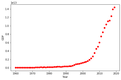

We can see that the growth starts off slow. Then, from 2005 onwards, the growth is very significant. It decelerates slightly after the period of the 2008 global recession.

Choosing a model

Looking at the plot, a logistic function would be a good approximation, since it has the property of starting with a slow growth, increasing growth in the middle, and then decreasing again at the end.
Let’s check this assumption below:

X = np.arange(-5.0, 5.0, 0.1)
Y = 1.0 / (1.0 + np.exp(-X))

plt.plot(X, Y)
plt.ylabel('Dependent Variable')
plt.xlabel('Independent Variable')
plt.show()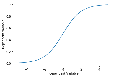

Build the model

Let’s build our regression model and initialize its parameters.

def sigmoid(x, Beta_1, Beta_2):
  y = 1/ (1 + np.exp(-Beta_1 * (x - Beta_2)))
  return y

Let’s look at a sample sigmoid line that might fit with the data.

beta_1 = 0.1
beta_2 = 1990

# logistic function
Y_pred = sigmoid(x_data, beta_1, beta_2)

# plot initial prediction againts data points
plt.plot(x_data, Y_pred*15000000000000)
plt.plot(x_data, y_data, 'ro')

[<matplotlib.lines.Line2D at 0x7f5c93a4d780>]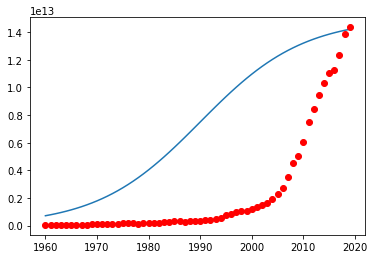

Our task is to find the best parameters for the model.
First, lets normalize our x and y.

xdata = x_data / max(x_data)
ydata = y_data / max(y_data)

How can we find the best parameters for our fit line?
We can use curve_fit, which uses non-linear least squares to fit our sigmoid function to the data.

from scipy.optimize import curve_fit
popt, pcov = curve_fit(sigmoid, xdata, ydata)

# print the final parameters
print('beta_1=%f, beta_2=%f' % (popt[0], popt[1]))

beta_1 = 571.415035, beta_2 = 0.995885

Plot the model

# plot the resulting regression model
x = np.linspace(1960, 2015, 55)
x = x/max(x)
plt.figure(figsize=(8,5))
y = sigmoid(x, *popt)
plt.plot(xdata, ydata, 'ro', label='data')
plt.plot(x, y, linewidth=3.0, label='fit')
plt.legend(loc='best')
plt.ylabel('GDP')
plt.xlabel('Year')
plt.show()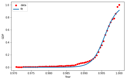

Train/Test Split the data

Split data into training and testing sets.

msk = np.random.randn(len(df)) < 0.8
train_x = x_data[msk]
test_x = xdata[~msk]
train_y = y_data[msk]
test_y = ydata[~msk]

Build the model using the train set.

popt, pcov = curve_fit(sigmoid, train_x, train_y)

/usr/local/lib/python3.6/dist-packages/scipy/optimize/minpack.py:808: OptimizeWarning: Covariance of the parameters could not be estimated
  category=OptimizeWarning)

Predict GDP using the test set.

y_hat = sigmoid(test_x, *popt)

Evaluate the model

print('Mean absolute error: %.2f' % np.mean(np.absolute(y_hat - test_y)))
print('Residual sum of error (MSE): %.2f' % np.mean((y_hat - test_y)**2))

from sklearn.metrics import r2_score
print('R2-score: %.2f' % r2_score(y_hat, test_y))

Mean absolute error: 0.40
Residual sum of error (MSE): 0.17
R2-score: -34427.16