In this blog post, we’ll try to figure out what breed of pet is shown in each image of a dataset.
The dataset we’ll be using is the Oxford-IIIT Pet dataset. It’s a 37 category pet dataset with roughly 200 images for each class. The images have a large variations in scale, pose and lighting. The dataset can be downloaded here.
First, let’s install fastai and import all its modules.
!pip install -Uqq fastbook
import fastbook
fastbook.setup_book()
[K |████████████████████████████████| 727kB 17.1MB/s
[K |████████████████████████████████| 1.2MB 47.1MB/s
[K |████████████████████████████████| 51kB 6.8MB/s
[K |████████████████████████████████| 194kB 56.0MB/s
[K |████████████████████████████████| 61kB 8.7MB/s
[K |████████████████████████████████| 51kB 7.8MB/s
[K |████████████████████████████████| 12.8MB 251kB/s
[K |████████████████████████████████| 776.8MB 23kB/s
[31mERROR: torchtext 0.9.0 has requirement torch==1.8.0, but you'll have torch 1.7.1 which is incompatible.[0m
[?25hMounted at /content/gdrivefrom fastbook import *from fastai.vision.all import *We’ll use untar_data to download files from a URL. We’ll set a path to this dataset.
path = untar_data(URLs.PETS)The below code helps us by showing only the relevant paths, and not showing the parent path folders.
Path.BASE_PATH = pathLet’s see what’s in the directory.
path.ls()(#2) [Path('images'),Path('annotations')]The dataset provides us with the images and annotations directories. The website for the dataset tells us that the annotations directory contains information about where the pets are rather than what they are. Hence, we will ignore the annotations directory.
Let’s look at the images directory.
(path/'images').ls()(#7393) [Path('images/german_shorthaired_99.jpg'),Path('images/boxer_88.jpg'),Path('images/great_pyrenees_119.jpg'),Path('images/Abyssinian_146.jpg'),Path('images/newfoundland_197.jpg'),Path('images/english_cocker_spaniel_161.jpg'),Path('images/British_Shorthair_269.jpg'),Path('images/newfoundland_139.jpg'),Path('images/Egyptian_Mau_221.jpg'),Path('images/havanese_108.jpg')...]There are 7,393 images in the folder. The breed of the pet is embedded in the image name along with a number and the extension. So, we can use a regular expression to extract the valuable information.
Let’s try out an example first.
We’ll pick one the filenames.
fname = (path/'images').ls()[0]re.findall(r'(.+)_\d+.jpg', fname.name)['german_shorthaired']This regular expression plucks out all the characters leading up to the last underscore character, as long as the subsequence chracters are numerical digits and then the JPEG file extension.
Now that we have confirmed that the regular expression works for the example, let’s use it to label the whole dataset. For labeling with regular expressions, we’ll use the RegexLabeller class.
pets = DataBlock(blocks = (ImageBlock, CategoryBlock),
                 get_items=get_image_files,
                 splitter=RandomSplitter(seed=42),
                 get_y=using_attr(RegexLabeller(r'(.+)_\d+.jpg'), 'name'),
                 item_tfms=Resize(460),
                 batch_tfms=aug_transforms(size=224, min_scale=0.75))

dls = pets.dataloaders(path/'images')
Let’s find out what breeds are present in the dataset.
dls.vocab['Abyssinian', 'Bengal', 'Birman', 'Bombay', 'British_Shorthair', 'Egyptian_Mau', 'Maine_Coon', 'Persian', 'Ragdoll', 'Russian_Blue', 'Siamese', 'Sphynx', 'american_bulldog', 'american_pit_bull_terrier', 'basset_hound', 'beagle', 'boxer', 'chihuahua', 'english_cocker_spaniel', 'english_setter', 'german_shorthaired', 'great_pyrenees', 'havanese', 'japanese_chin', 'keeshond', 'leonberger', 'miniature_pinscher', 'newfoundland', 'pomeranian', 'pug', 'saint_bernard', 'samoyed', 'scottish_terrier', 'shiba_inu', 'staffordshire_bull_terrier', 'wheaten_terrier', 'yorkshire_terrier']dls.show_batch(max_n=9, figsize=(6,7))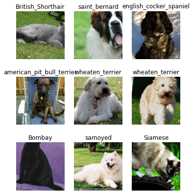
Training a simple model
Let’s train a simple model. We’ll be using transfer learning to train the model using the ImageNet dataset. The fastai method fine_tune will help us with this.
learn = cnn_learner(dls, resnet34, metrics=error_rate)
learn.fine_tune(15)
Downloading: "https://download.pytorch.org/models/resnet34-333f7ec4.pth" to /root/.cache/torch/hub/checkpoints/resnet34-333f7ec4.pth
HBox(children=(FloatProgress(value=0.0, max=87306240.0), HTML(value='')))| epoch | train_loss | valid_loss | error_rate | time |
|---|---|---|---|---|
| 0 | 1.541179 | 1.021038 | 0.307848 | 01:09 |
| epoch | train_loss | valid_loss | error_rate | time |
|---|---|---|---|---|
| 0 | 0.476121 | 0.846739 | 0.263870 | 01:12 |
| 1 | 0.359381 | 0.908805 | 0.273342 | 01:12 |
| 2 | 0.305826 | 0.898781 | 0.263870 | 01:12 |
| 3 | 0.285199 | 0.767794 | 0.236130 | 01:12 |
| 4 | 0.242656 | 0.810228 | 0.234100 | 01:12 |
| 5 | 0.187951 | 0.887635 | 0.228687 | 01:12 |
| 6 | 0.151485 | 0.777132 | 0.217862 | 01:12 |
| 7 | 0.136154 | 0.763384 | 0.197564 | 01:13 |
| 8 | 0.105534 | 0.732230 | 0.200271 | 01:12 |
| 9 | 0.084376 | 0.664226 | 0.173884 | 01:11 |
| 10 | 0.058460 | 0.670688 | 0.181326 | 01:12 |
| 11 | 0.038214 | 0.669005 | 0.180650 | 01:11 |
| 12 | 0.023151 | 0.693375 | 0.177267 | 01:11 |
| 13 | 0.024510 | 0.665506 | 0.170501 | 01:11 |
| 14 | 0.023619 | 0.637721 | 0.161028 | 01:11 |
Let’s look at a graph of the training and validation loss.
learn.recorder.plot_loss()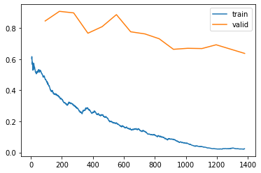
Even our simple model gives us really good accuracy. Let’s use a classification matrix to interpret our model; see where it’s doing well and where it’s doing badly.
interp = ClassificationInterpretation.from_learner(learn)
interp.plot_confusion_matrix(figsize=(12,12), dpi=60)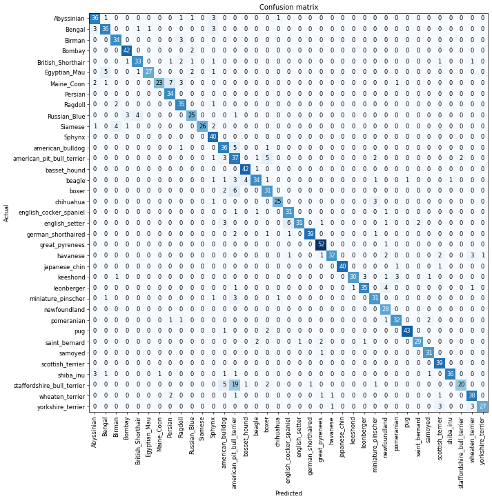
We have 37 different breeds of pet, which means we have 37 X 37 entries in this matrix, which makes it hard to interpret. We’ll use the most_confused method, which just shows us the cells of the confusion matrix with the most incorrect predictions.
# cells with 5 or more incorrect predictions
interp.most_confused(min_val=5)
[('staffordshire_bull_terrier', 'american_pit_bull_terrier', 19),
('Maine_Coon', 'Persian', 7),
('boxer', 'american_pit_bull_terrier', 6),
('english_setter', 'english_cocker_spaniel', 6),
('Egyptian_Mau', 'Bengal', 5),
('american_bulldog', 'american_pit_bull_terrier', 5),
('american_pit_bull_terrier', 'boxer', 5),
('staffordshire_bull_terrier', 'american_bulldog', 5)]These are the breeds of cats and dogs that are hardest to predict by our model. Coincidently, these are also pretty common comparisons that even experts get confused about, for e.g. the differences in appearance between the Staffordshire Bull Terrier and the American Pit Bull Terrier (i.e. the comparison that confused our model the most) are so minute that most humans will find it hard to distinguish them.
interp.plot_top_losses(8, nrows=2)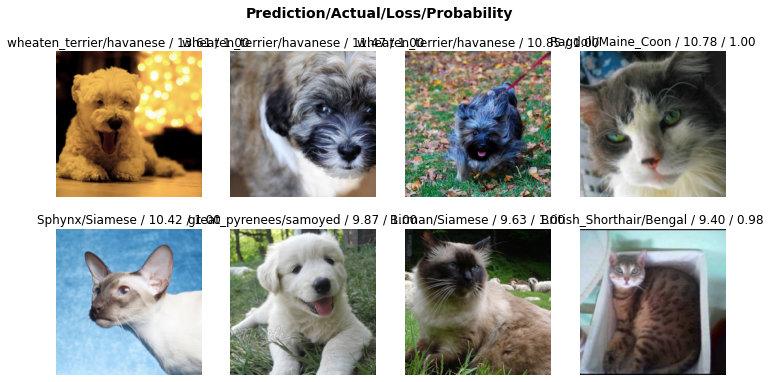
learn.show_results()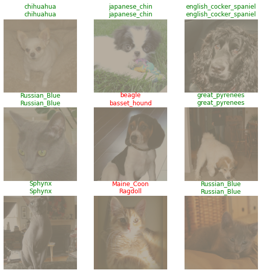
Let’s save this model.
learn.save('model1')Path('models/model1.pth')Picking the Learning Rate
Let’s use fastai’s learning rate finder to find a suitable learning rate.
learn2 = cnn_learner(dls, resnet34, metrics=error_rate)
lr_min, lr_steep = learn2.lr_find()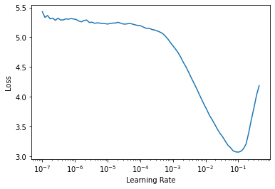
print(f'Minimum/10: {lr_min: .2e}, steepest_point: {lr_steep: .2e}')Minimum/10: 1.00e-02, steepest_point: 5.25e-03Let’s now pick the learning rate at the steepest point in the graph.
learn2 = cnn_learner(dls, resnet34, metrics=error_rate)
learn2.fine_tune(15, 5.25e-3)| epoch | train_loss | valid_loss | error_rate | time |
|---|---|---|---|---|
| 0 | 1.105870 | 1.111952 | 0.329499 | 01:13 |
| epoch | train_loss | valid_loss | error_rate | time |
|---|---|---|---|---|
| 0 | 0.409039 | 0.954296 | 0.280785 | 01:16 |
| 1 | 0.338957 | 1.197951 | 0.326116 | 01:17 |
| 2 | 0.374680 | 1.036932 | 0.278755 | 01:17 |
| 3 | 0.444182 | 1.355077 | 0.357240 | 01:16 |
| 4 | 0.408214 | 1.485182 | 0.407307 | 01:16 |
| 5 | 0.353418 | 1.045590 | 0.292963 | 01:17 |
| 6 | 0.321617 | 1.315597 | 0.347767 | 01:16 |
| 7 | 0.277381 | 0.998754 | 0.297023 | 01:16 |
| 8 | 0.186780 | 0.957907 | 0.265900 | 01:17 |
| 9 | 0.117437 | 0.792308 | 0.219215 | 01:17 |
| 10 | 0.099135 | 0.933071 | 0.249662 | 01:17 |
| 11 | 0.060645 | 0.753601 | 0.200947 | 01:16 |
| 12 | 0.040250 | 0.736492 | 0.197564 | 01:16 |
| 13 | 0.034840 | 0.737214 | 0.198241 | 01:16 |
| 14 | 0.023275 | 0.721530 | 0.194181 | 01:16 |
Let’s plot the losses on a graph.
learn2.recorder.plot_loss()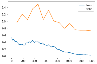
learn2.save('model2')Path('models/model2.pth')Unfreezing and Transfer Learning
When fine-tuning, we aim to replace the random weights in our added linear layers with weights that correctly achieve our desired task of classifying pet breeds without breaking the carefully pretrained weights and the other layers. We’ll tell the optimizer to only update the weights in those randomly added final layers, and not change the weights in the rest of the neural network. This is called freezing the pretrained layers.
When we create a model from a pretrained network, fastai automatically freexzes all of the pretrained layers for us.
We can try and improve our model by changing the parameters of the fine_tune method.
First, we’ll train the randomly added layers for three epochs, using fit_one_cycle, which is the suggested way to train models without using fine_tune.
learn3 = cnn_learner(dls, resnet34, metrics=error_rate)
learn3.fit_one_cycle(4, 5.25e-3)| epoch | train_loss | valid_loss | error_rate | time |
|---|---|---|---|---|
| 0 | 1.082502 | 1.659888 | 0.414073 | 01:11 |
| 1 | 0.648850 | 1.761306 | 0.445873 | 01:12 |
| 2 | 0.421008 | 1.299498 | 0.379567 | 01:11 |
| 3 | 0.278318 | 0.959298 | 0.298376 | 01:11 |
Now, we’ll unfreeze the model.
learn3.unfreeze()We’ll run lr_find again because having more layers to train, and weights that have already been trained for three epochs, means our previously found learning rate isn’t appropriate anymore.
learn3.lr_find()SuggestedLRs(lr_min=1.58489319801447e-07, lr_steep=1.3182567499825382e-06)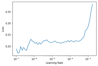
We can see that we have a somewhat flat area before a sharp increase, and we should take a point well before that sharp increase. But the deepest layers of our pretrained model might not need as high a learning rate as the last ones, so we should use different learning rates for different layers, which is known as discriminative learning rates.
We’ll use a lower learning rate for the early layers of the neural network, and a higher learning rate for the later layers (and especially the randomly added layers).
fastai lets you pass a Python slice object anywhere that a learning rate is expected. The first value passed will be the learning rate in the earliest layer of the neural network, and the second value will be the learning rate in the final layer. The layers in between will have learning rates that are multiplicatively equidistant throughout that range.
learn3 = cnn_learner(dls, resnet34, metrics=error_rate)
learn3.fit_one_cycle(4, 5.25e-3)
learn3.unfreeze()
learn3.fit_one_cycle(12, lr_max=slice(1e-6,1e-4))| epoch | train_loss | valid_loss | error_rate | time |
|---|---|---|---|---|
| 0 | 1.090194 | 1.388986 | 0.393099 | 01:12 |
| 1 | 0.649271 | 1.753144 | 0.456698 | 01:12 |
| 2 | 0.439216 | 1.004193 | 0.300406 | 01:12 |
| 3 | 0.294163 | 0.960151 | 0.284168 | 01:12 |
| epoch | train_loss | valid_loss | error_rate | time |
|---|---|---|---|---|
| 0 | 0.233927 | 0.932793 | 0.276725 | 01:17 |
| 1 | 0.212731 | 0.892106 | 0.260487 | 01:18 |
| 2 | 0.203497 | 0.919420 | 0.273342 | 01:18 |
| 3 | 0.197853 | 0.822041 | 0.249662 | 01:17 |
| 4 | 0.183791 | 0.815729 | 0.244249 | 01:18 |
| 5 | 0.161308 | 0.875792 | 0.261840 | 01:17 |
| 6 | 0.146391 | 0.858144 | 0.253721 | 01:17 |
| 7 | 0.129562 | 0.838909 | 0.255751 | 01:16 |
| 8 | 0.126738 | 0.844979 | 0.251691 | 01:17 |
| 9 | 0.123629 | 0.839640 | 0.253721 | 01:16 |
| 10 | 0.124569 | 0.803057 | 0.238836 | 01:17 |
| 11 | 0.112034 | 0.806164 | 0.238836 | 01:18 |
learn3.recorder.plot_loss()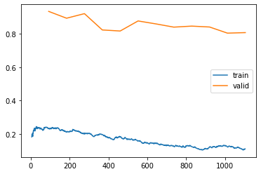
learn3.save('model3')Path('models/model3.pth')Using Deeper Architectures
Let’s try to improve our model’s performance using deeper architectures.
Deeper architectures like ResNet50 take longer to train. We can speed things up by using mixed-precision training, wherein we can use less-precise numbers like fp16 (half-precision floating point). To enable this feature, we just add to_fp16() to the Learner.
# import the fp16 module
from fastai.callback.fp16 import *
learn4 = cnn_learner(dls, resnet50, metrics=error_rate).to_fp16()
learn4.fine_tune(15)Downloading: "https://download.pytorch.org/models/resnet50-19c8e357.pth" to /root/.cache/torch/hub/checkpoints/resnet50-19c8e357.pth
HBox(children=(FloatProgress(value=0.0, max=102502400.0), HTML(value='')))| epoch | train_loss | valid_loss | error_rate | time |
|---|---|---|---|---|
| 0 | 0.994141 | 1.132718 | 0.330176 | 01:07 |
| epoch | train_loss | valid_loss | error_rate | time |
|---|---|---|---|---|
| 0 | 0.350162 | 0.960766 | 0.280785 | 01:09 |
| 1 | 0.258597 | 0.936031 | 0.276725 | 01:08 |
| 2 | 0.256309 | 0.948686 | 0.282815 | 01:09 |
| 3 | 0.253626 | 1.049184 | 0.276725 | 01:08 |
| 4 | 0.251305 | 1.222372 | 0.322057 | 01:09 |
| 5 | 0.179732 | 1.153965 | 0.279432 | 01:09 |
| 6 | 0.142337 | 1.300296 | 0.315968 | 01:09 |
| 7 | 0.121877 | 0.982640 | 0.244249 | 01:10 |
| 8 | 0.097359 | 1.028661 | 0.261840 | 01:10 |
| 9 | 0.071566 | 0.761003 | 0.196211 | 01:09 |
| 10 | 0.036808 | 0.773423 | 0.196888 | 01:10 |
| 11 | 0.029443 | 0.626214 | 0.165088 | 01:09 |
| 12 | 0.022480 | 0.700238 | 0.184709 | 01:09 |
| 13 | 0.018170 | 0.660072 | 0.177267 | 01:09 |
| 14 | 0.013801 | 0.684406 | 0.177943 | 01:09 |
learn4.recorder.plot_loss()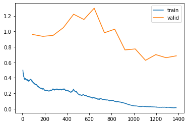
learn4.save('model4')Path('models/model4.pth')Exporting our model
Comparing the training results and the graphs of the losses, we can conclude that the first model we trained was the best one. So we will now export this model and create a GUI and build a classifer within our notebook itself.
learn.export()path = Path()
path.ls(file_exts='.pkl')(#1) [Path('export.pkl')]learn_inf = load_learner('export.pkl')learn_inf.dls.vocab['Abyssinian', 'Bengal', 'Birman', 'Bombay', 'British_Shorthair', 'Egyptian_Mau', 'Maine_Coon', 'Persian', 'Ragdoll', 'Russian_Blue', 'Siamese', 'Sphynx', 'american_bulldog', 'american_pit_bull_terrier', 'basset_hound', 'beagle', 'boxer', 'chihuahua', 'english_cocker_spaniel', 'english_setter', 'german_shorthaired', 'great_pyrenees', 'havanese', 'japanese_chin', 'keeshond', 'leonberger', 'miniature_pinscher', 'newfoundland', 'pomeranian', 'pug', 'saint_bernard', 'samoyed', 'scottish_terrier', 'shiba_inu', 'staffordshire_bull_terrier', 'wheaten_terrier', 'yorkshire_terrier']from fastai.vision.widgets import *def on_click_classify(change):
img = PILImage.create(btn_upload.data[-1])
out_pl.clear_output()
with out_pl: display(img.to_thumb(128,128))
pred,pred_idx,probs = learn_inf.predict(img)
lbl_pred.value = f'Prediction: {pred}; Probability: {probs[pred_idx]:.04f}'
btn_run.on_click(on_click_classify)VBox([widgets.Label('Select your pet!'),
btn_upload, btn_run, out_pl, lbl_pred])VBox(children=(Label(value='Select your pet!'), FileUpload(value={'pet_dog.jpg': {'metadata': {'lastModified':…