Imagine that you have a customer dataset, and you are interested in exploring the behavior of your customers using their historical data.
Customer segmentation is the practice of partitioning a customer base into groups of individuals that have similar characteristics. It is a significant strategy as a business can target these specific groups of customers and effectively allocate marketing resources.
The dataset being worked on consists of 850 customers, with information about their income and debt. You can download the data set here: https://cocl.us/customer_dataset
import random # library for random number generation
import numpy as np # library for vectorized computation
import pandas as pd # library to process data as dataframes

import matplotlib.pyplot as plt # plotting library
# backend for rendering plots within the browser
%matplotlib inline

from sklearn.cluster import KMeans
from sklearn.datasets.samples_generator import make_blobs

print('Libraries imported.')
Libraries imported.Read the data into a pandas dataframe.
customers_df = pd.read_csv('Cust_Segmentation.csv')
customers_df.head()| Customer Id | Age | Edu | Years Employed | Income | Card Debt | Other Debt | Defaulted | Address | DebtIncomeRatio | |
|---|---|---|---|---|---|---|---|---|---|---|
| 0 | 1 | 41 | 2 | 6 | 19 | 0.124 | 1.073 | 0.0 | NBA001 | 6.3 |
| 1 | 2 | 47 | 1 | 26 | 100 | 4.582 | 8.218 | 0.0 | NBA021 | 12.8 |
| 2 | 3 | 33 | 2 | 10 | 57 | 6.111 | 5.802 | 1.0 | NBA013 | 20.9 |
| 3 | 4 | 29 | 2 | 4 | 19 | 0.681 | 0.516 | 0.0 | NBA009 | 6.3 |
| 4 | 5 | 47 | 1 | 31 | 253 | 9.308 | 8.908 | 0.0 | NBA008 | 7.2 |
Preprocessing the data
Address in this dataset is a categorical variable. k-means algorithm isn’t directly applicable to categorical variables because the Euclidean distance function isn’t really meaningful for discrete variables.
So let’s drop this feature and run clustering.
df = customers_df.drop('Address', axis=1)
df.head()| Customer Id | Age | Edu | Years Employed | Income | Card Debt | Other Debt | Defaulted | DebtIncomeRatio | |
|---|---|---|---|---|---|---|---|---|---|
| 0 | 1 | 41 | 2 | 6 | 19 | 0.124 | 1.073 | 0.0 | 6.3 |
| 1 | 2 | 47 | 1 | 26 | 100 | 4.582 | 8.218 | 0.0 | 12.8 |
| 2 | 3 | 33 | 2 | 10 | 57 | 6.111 | 5.802 | 1.0 | 20.9 |
| 3 | 4 | 29 | 2 | 4 | 19 | 0.681 | 0.516 | 0.0 | 6.3 |
| 4 | 5 | 47 | 1 | 31 | 253 | 9.308 | 8.908 | 0.0 | 7.2 |
Normalize the dataset using StandardScalar(). Normalization is a statistical method that helps mathematical-based algorithms interpret features with different magnitudes and distributions equally.
from sklearn.preprocessing import StandardScaler

X = df.values[:,1:]
X = np.nan_to_num(X)
cluster_dataset = StandardScaler().fit_transform(X)
cluster_dataset
array([[ 0.74291541, 0.31212243, -0.37878978, ..., -0.59048916,
-0.52379654, -0.57652509],
[ 1.48949049, -0.76634938, 2.5737211 , ..., 1.51296181,
-0.52379654, 0.39138677],
[-0.25251804, 0.31212243, 0.2117124 , ..., 0.80170393,
1.90913822, 1.59755385],
...,
[-1.24795149, 2.46906604, -1.26454304, ..., 0.03863257,
1.90913822, 3.45892281],
[-0.37694723, -0.76634938, 0.50696349, ..., -0.70147601,
-0.52379654, -1.08281745],
[ 2.1116364 , -0.76634938, 1.09746566, ..., 0.16463355,
-0.52379654, -0.2340332 ]])Modeling
Let’s run our model and group the customers into three clusters.
num_clusters = 3

k_means = KMeans(init='k-means++', n_clusters=num_clusters, n_init=12)
k_means.fit(cluster_dataset)
labels = k_means.labels_
print(labels)
[1 2 0 1 2 2 1 1 1 2 0 1 1 1 0 1 1 1 2 1 1 1 0 2 2 1 1 1 1 1 1 2 0 1 1 1 0
0 1 2 0 2 1 2 1 2 1 1 1 1 2 2 0 1 0 0 0 1 1 1 2 1 2 2 1 1 1 0 1 0 1 1 1 1
1 1 1 1 2 1 1 0 2 1 2 1 1 1 0 0 1 1 0 0 1 1 1 1 0 1 0 2 1 0 0 2 1 1 1 1 1
1 1 0 1 1 1 1 2 1 1 1 1 1 1 1 1 1 1 1 1 1 1 1 1 1 1 1 1 0 0 1 1 1 2 1 1 0
1 1 1 2 0 1 1 1 1 2 0 0 1 2 1 1 1 1 1 1 1 1 2 1 1 0 1 0 1 1 0 2 0 1 1 2 0
2 1 1 1 1 1 2 1 0 1 1 1 2 2 1 2 1 0 1 1 0 1 2 1 0 1 1 1 1 1 0 0 2 1 1 0 2
1 1 1 1 2 1 1 0 1 1 1 1 2 1 1 0 2 1 1 1 1 1 1 2 1 2 1 1 1 1 1 1 2 0 1 0 1
1 1 2 1 0 2 0 1 2 1 1 0 1 1 1 1 0 0 0 1 1 1 2 1 1 2 1 2 1 1 2 1 1 1 0 1 1
0 1 0 2 1 1 1 1 0 1 1 0 0 1 1 1 1 1 1 1 1 0 1 0 2 1 0 1 1 1 0 0 1 1 1 2 0
1 1 0 1 2 1 1 1 1 1 0 2 1 1 1 1 1 2 1 1 1 1 1 2 1 1 1 2 0 1 0 1 1 1 2 2 1
0 1 2 0 0 1 1 1 0 1 1 1 1 1 2 1 2 1 1 1 1 0 1 0 1 1 1 2 1 1 1 1 0 1 1 0 0
2 1 1 1 1 1 0 0 1 2 0 2 1 1 0 1 1 2 2 1 0 1 1 2 1 0 1 2 1 1 1 2 1 1 1 1 2
1 0 1 1 1 1 2 0 1 1 2 1 0 1 1 2 1 2 1 1 1 1 1 1 1 2 2 1 1 2 1 0 1 1 1 0 1
0 1 1 1 1 1 2 0 0 1 2 1 2 1 1 0 2 1 0 0 0 2 2 0 1 1 0 1 0 0 1 0 2 1 1 0 1
0 2 0 1 1 0 1 1 0 0 0 1 1 1 2 2 1 1 0 1 1 0 2 1 0 1 1 1 0 1 2 1 2 2 1 2 1
1 2 1 0 1 1 1 1 0 0 1 2 1 2 1 1 2 1 0 1 0 1 0 0 0 2 0 1 1 1 0 1 1 1 2 1 2
1 0 0 1 1 1 1 1 1 1 0 2 1 2 1 1 0 1 1 1 0 1 1 0 0 0 0 1 2 1 0 0 1 1 1 1 2
2 1 0 1 1 2 1 1 2 1 2 1 1 2 0 2 2 2 0 1 1 0 1 2 2 1 1 1 2 0 1 1 1 1 2 1 1
1 1 1 0 1 1 2 1 1 2 1 1 1 1 1 1 0 2 1 1 0 1 1 1 1 0 1 2 1 1 2 1 1 0 1 0 1
0 0 1 1 1 2 0 2 1 2 2 1 0 1 2 1 2 1 1 1 1 1 2 1 0 1 1 2 2 1 1 2 1 1 1 1 1
1 1 1 0 1 1 2 1 1 1 1 1 1 1 0 1 1 1 2 0 2 2 1 1 1 0 1 1 1 0 0 1 0 1 1 1 2
1 1 1 1 1 1 1 2 1 1 1 1 1 1 2 2 0 0 1 0 1 1 1 1 2 0 1 1 1 1 1 2 0 1 1 1 0
1 1 0 1 1 1 1 1 1 0 0 2 2 1 1 1 0 1 1 1 1 1 1 1 1 1 1 1 1 1 1 1 1 0 1 2]Insights
Each row in the dataset represents a customer, and therefore, each row is assigned a label.
df['Labels'] = labels
df.head()| Customer Id | Age | Edu | Years Employed | Income | Card Debt | Other Debt | Defaulted | DebtIncomeRatio | Labels | |
|---|---|---|---|---|---|---|---|---|---|---|
| 0 | 1 | 41 | 2 | 6 | 19 | 0.124 | 1.073 | 0.0 | 6.3 | 1 |
| 1 | 2 | 47 | 1 | 26 | 100 | 4.582 | 8.218 | 0.0 | 12.8 | 2 |
| 2 | 3 | 33 | 2 | 10 | 57 | 6.111 | 5.802 | 1.0 | 20.9 | 0 |
| 3 | 4 | 29 | 2 | 4 | 19 | 0.681 | 0.516 | 0.0 | 6.3 | 1 |
| 4 | 5 | 47 | 1 | 31 | 253 | 9.308 | 8.908 | 0.0 | 7.2 | 2 |
Check the centroid values by averaging the features in each cluster.
df.groupby('Labels').mean()| Customer Id | Age | Edu | Years Employed | Income | Card Debt | Other Debt | Defaulted | DebtIncomeRatio | |
|---|---|---|---|---|---|---|---|---|---|
| Labels | |||||||||
| 0 | 424.451807 | 31.891566 | 1.861446 | 3.963855 | 31.789157 | 1.576675 | 2.843355 | 0.993939 | 13.994578 |
| 1 | 426.122905 | 33.817505 | 1.603352 | 7.625698 | 36.143389 | 0.853128 | 1.816855 | 0.000000 | 7.964991 |
| 2 | 424.408163 | 43.000000 | 1.931973 | 17.197279 | 101.959184 | 4.220673 | 7.954483 | 0.162393 | 13.915646 |
Let’s look at the distribution of customers based on their age and income.
area = np.pi * ( X[:, 1])**2
plt.scatter(X[:, 0], X[:, 3], s=area, c=labels.astype(np.float), alpha=0.5)
plt.xlabel('Age', fontsize=16)
plt.ylabel('Income', fontsize=16)
plt.show()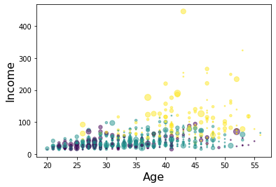
from mpl_toolkits.mplot3d import Axes3D
fig = plt.figure(1, figsize=(8, 6))
plt.clf()
ax = Axes3D(fig, rect=[0, 0, .95, 1], elev=48, azim=134)

plt.cla()
ax.set_xlabel('Age')
ax.set_ylabel('Income')
ax.set_zlabel('DebtIncomeRatio')

ax.scatter(X[:, 1], X[:, 0], X[:, 3], c= labels.astype(np.float))
<mpl_toolkits.mplot3d.art3d.Path3DCollection at 0x1a21784a90>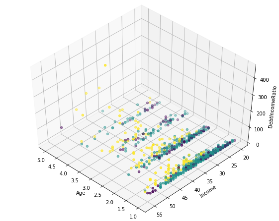
k-means will partition the customers into three groups since we specified the algorithm to generate three clusters. The customers in each cluster are similar to each other in terms of the features included in the dataset.
We can create a profile for each group, considering the common characteristics of each cluster. For example, the three clusters can be: - older, high income, and indebted - middle-aged, middle income, and financially responsible - young, low income, and indebted
You can devise your own profiles based on the means above and come up with labels that you think best describe each cluster.