We will build a classifier to predict the class of new or unknown customers for a telecommunications provider. We will use a specific type of classification called K-Nearest Neighbors.
Imagine a telecommunications provider has segmented its customer base by service usage patterns, categorizing the customers into four groups. If demographic data can be used to predict group membership, the company can customize offers for individual prospective customers. It is a classification problem. That is, given the dataset, with predefined labels, we need to build a model to be used to predict class of a new or unknown case.
The example focuses on using demographic data, such as region, age, and marital, to predict usage patterns.
The target field, called custcat, has four possible values that correspond to the four customer groups, as follows: - 1- Basic Service - 2- E-Service - 3- Plus Service - 4- Total Service
In this blog post, we will build a classifier to predict the class of unknown cases. We will use a specific type of classification called K-Nearest Neighbors.
K-Nearest Neighbors is an algorithm for supervised learning, where the data is trained with data points corresponding to their classification. Once a point is predicted, it takes into account the ‘K’ nearest points to it to determine its classification.
# import libraries
import itertools
import numpy as np
import matplotlib.pyplot as plt
from matplotlib.ticker import NullFormatter
import pandas as pd
from sklearn import preprocessing
%matplotlib inline
# read the data into a pandas dataframe
df = pd.read_csv('teleCust1000t.csv')
df.head()|
|
region |
tenure |
age |
marital |
address |
income |
ed |
employ |
retire |
gender |
reside |
custcat |
|---|---|---|---|---|---|---|---|---|---|---|---|---|
|
0 |
2 |
13 |
44 |
1 |
9 |
64.0 |
4 |
5 |
0.0 |
0 |
2 |
1 |
|
1 |
3 |
11 |
33 |
1 |
7 |
136.0 |
5 |
5 |
0.0 |
0 |
6 |
4 |
|
2 |
3 |
68 |
52 |
1 |
24 |
116.0 |
1 |
29 |
0.0 |
1 |
2 |
3 |
|
3 |
2 |
33 |
33 |
0 |
12 |
33.0 |
2 |
0 |
0.0 |
1 |
1 |
1 |
|
4 |
2 |
23 |
30 |
1 |
9 |
30.0 |
1 |
2 |
0.0 |
0 |
4 |
3 |
Analyze the data
# dimensions of data
df.shape
(1000, 12)How many customers of each class are present in the dataset?
df['custcat'].value_counts()3 281
1 266
4 236
2 217
Name: custcat, dtype: int64There are - 281 customers in the ‘Plus Service’ category - 266 in the ‘Basic Service’ category - 236 in the ‘Total Service’ category - 217 in the ‘E-Service’ category.
Explore the data using histograms.
viz = df[['income', 'age', 'employ', 'reside']]
viz.hist()
plt.show()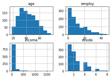
Define the feature set, X.
df.columnsIndex(['region', 'tenure', 'age', 'marital', 'address', 'income', 'ed',
'employ', 'retire', 'gender', 'reside', 'custcat'],
dtype='object')To use the scikit-learn library, convert the Pandas dataframe to a Numpy array.
X = df[['region', 'tenure', 'age', 'marital', 'address', 'income', 'ed',
       'employ', 'retire', 'gender', 'reside']].values
X[0:5]
array([[ 2., 13., 44., 1., 9., 64., 4., 5., 0., 0., 2.],
[ 3., 11., 33., 1., 7., 136., 5., 5., 0., 0., 6.],
[ 3., 68., 52., 1., 24., 116., 1., 29., 0., 1., 2.],
[ 2., 33., 33., 0., 12., 33., 2., 0., 0., 1., 1.],
[ 2., 23., 30., 1., 9., 30., 1., 2., 0., 0., 4.]])# the label
y = df['custcat'].values
y[0:5]array([1, 4, 3, 1, 3], dtype=int64)Normalize the data
X = preprocessing.StandardScaler().fit(X).transform(X.astype(float))
X[0:5]
array([[-0.02696767, -1.055125 , 0.18450456, 1.0100505 , -0.25303431,
-0.12650641, 1.0877526 , -0.5941226 , -0.22207644, -1.03459817,
-0.23065004],
[ 1.19883553, -1.14880563, -0.69181243, 1.0100505 , -0.4514148 ,
0.54644972, 1.9062271 , -0.5941226 , -0.22207644, -1.03459817,
2.55666158],
[ 1.19883553, 1.52109247, 0.82182601, 1.0100505 , 1.23481934,
0.35951747, -1.36767088, 1.78752803, -0.22207644, 0.96655883,
-0.23065004],
[-0.02696767, -0.11831864, -0.69181243, -0.9900495 , 0.04453642,
-0.41625141, -0.54919639, -1.09029981, -0.22207644, 0.96655883,
-0.92747794],
[-0.02696767, -0.58672182, -0.93080797, 1.0100505 , -0.25303431,
-0.44429125, -1.36767088, -0.89182893, -0.22207644, -1.03459817,
1.16300577]])Train/Test Split
from sklearn.model_selection import train_test_split
X_train, X_test, y_train, y_test = train_test_split(X, y, test_size=0.2, random_state=4)
print('Train set: ', X_train.shape, y_train.shape)
print('Test set: ', X_test.shape, y_test.shape)
Train set: (800, 11) (800,)
Test set: (200, 11) (200,)KNN Classification
# import library
from sklearn.neighbors import KNeighborsClassifier
Training
Let’s start the algorithm with k=4.
k = 4
neigh = KNeighborsClassifier(n_neighbors=k).fit(X_train, y_train)
neigh
KNeighborsClassifier(algorithm='auto', leaf_size=30, metric='minkowski',
metric_params=None, n_jobs=None, n_neighbors=4, p=2,
weights='uniform')Predicting
yhat = neigh.predict(X_test)
yhat[0:5]
array([1, 1, 3, 2, 4], dtype=int64)Evaluating
In multilabel classification, accuracy classification score is a function that computes subset accuracy. This function is equal to the jaccard_similarity_score function. Essentially, it calculates how closely the actual labels and predicted labels are matched in the test set.
from sklearn import metrics
print('Train set accuracy: ', metrics.accuracy_score(y_train, neigh.predict(X_train)))
print('Test set accuracy: ', metrics.accuracy_score(y_test, yhat))
Train set accuracy: 0.5475
Test set accuracy: 0.32Different K values
Calculate the accuracy of KNN for different K values.
Ks = 10
mean_acc = np.zeros((Ks-1))
std_acc = np.zeros((Ks-1))
ConfusionMx = [];
for n in range(1, Ks):
    # train model and predict
    neigh = KNeighborsClassifier(n_neighbors = n).fit(X_train, y_train)
    yhat = neigh.predict(X_test)
    mean_acc[n-1] = metrics.accuracy_score(y_test, yhat)
    std_acc[n-1] = np.std(yhat==y_test) / np.sqrt(yhat.shape[0])

mean_acc
array([0.3 , 0.29 , 0.315, 0.32 , 0.315, 0.31 , 0.335, 0.325, 0.34 ])Plot model accuracy for different number of Neighbors
plt.plot(range(1,Ks), mean_acc, 'g')
plt.fill_between(range(1,Ks), mean_acc - 1*std_acc,mean_acc + 1*std_acc, alpha=0.1)
plt.legend(('Accuracy ', '+/- 3xstd'))
plt.ylabel('Accuracy')
plt.xlabel('Number of Neighbors (K)')
plt.tight_layout()
plt.show()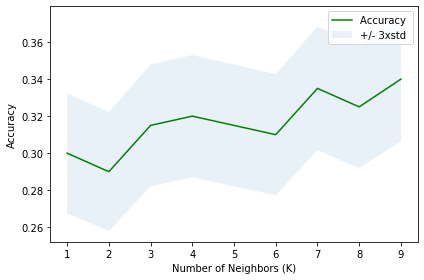
print('The best accuracy was with', mean_acc.max(), 'with k=', mean_acc.argmax()+1)The best accuracy was with 0.34 with k= 9Evaluate the above code with k=16.
# train
k = 9
neigh = KNeighborsClassifier(n_neighbors=k).fit(X_train, y_train)
neigh
KNeighborsClassifier(algorithm='auto', leaf_size=30, metric='minkowski',
metric_params=None, n_jobs=None, n_neighbors=9, p=2,
weights='uniform')# predict
yhat = neigh.predict(X_test)
yhat[0:5]array([3, 1, 3, 2, 4], dtype=int64)# evaluate
from sklearn import metrics
print('Train set accuracy: ', metrics.accuracy_score(y_train, neigh.predict(X_train)))
print('Test set accuracy: ', metrics.accuracy_score(y_test, yhat))Train set accuracy: 0.5025
Test set accuracy: 0.34