A telecommunications company is concerned about the number of customers leaving their landline business for cable competitors. They need to understand who is leaving. Imagine that you are an analyst at this company and you have to find out who is leaving and why. In this blog post, we will create a model for the telecommunications company using Logistic Regression to predict when its customers will leave for a competitor, so that they can take some action to retain the customers.
While Linear Regression is suited for estimating continuous values, it is not the best tool for predicting the class of an observed data point. In order to estimate the class of a data point, we need some sort of guidance on what would be the most probable class for that data point. For this, we use Logistic Regression.
Logistic Regression is a variation of Linear Regression, useful when the observed dependent variable, y, is categorical. It produces a formula that predicts the probability of the class label as a function of the independent variables. Logistic Regression fits a special s-shaped curve by taking the linear regression and transforming the numeric estimate into a probability.
The dataset we’ll be using contains information about 200 customers. It includes information about: - Customers who left within the last month - the column is called Churn. - Services that each customer has signed up for - phone, multiple lines, internet, online security, online backup, device protection, tech support, and streaming TV and movies. - Customer account information - how long they have been a customer, contract, payment method, paperless billing, monthly charges, and total charges. - Demographic information about customers - gender, age, range, and if they have partners and dependents.
Typically, it is less expensive to keep customers than to acquire new ones, so the focus of this analysis is to predict the customers who will stay with the company.
# import libraries
import pandas as pd
import numpy as np
import pylab as pl
import scipy.optimize as opt
import matplotlib.pyplot as plt
%matplotlib inline
# read the data into a pandas dataframe
df = pd.read_csv('ChurnData.csv')
df.head()| tenure | age | address | income | ed | employ | equip | callcard | wireless | longmon | … | pager | internet | callwait | confer | ebill | loglong | logtoll | lninc | custcat | churn | |
|---|---|---|---|---|---|---|---|---|---|---|---|---|---|---|---|---|---|---|---|---|---|
| 0 | 11.0 | 33.0 | 7.0 | 136.0 | 5.0 | 5.0 | 0.0 | 1.0 | 1.0 | 4.40 | … | 1.0 | 0.0 | 1.0 | 1.0 | 0.0 | 1.482 | 3.033 | 4.913 | 4.0 | 1.0 |
| 1 | 33.0 | 33.0 | 12.0 | 33.0 | 2.0 | 0.0 | 0.0 | 0.0 | 0.0 | 9.45 | … | 0.0 | 0.0 | 0.0 | 0.0 | 0.0 | 2.246 | 3.240 | 3.497 | 1.0 | 1.0 |
| 2 | 23.0 | 30.0 | 9.0 | 30.0 | 1.0 | 2.0 | 0.0 | 0.0 | 0.0 | 6.30 | … | 0.0 | 0.0 | 0.0 | 1.0 | 0.0 | 1.841 | 3.240 | 3.401 | 3.0 | 0.0 |
| 3 | 38.0 | 35.0 | 5.0 | 76.0 | 2.0 | 10.0 | 1.0 | 1.0 | 1.0 | 6.05 | … | 1.0 | 1.0 | 1.0 | 1.0 | 1.0 | 1.800 | 3.807 | 4.331 | 4.0 | 0.0 |
| 4 | 7.0 | 35.0 | 14.0 | 80.0 | 2.0 | 15.0 | 0.0 | 1.0 | 0.0 | 7.10 | … | 0.0 | 0.0 | 1.0 | 1.0 | 0.0 | 1.960 | 3.091 | 4.382 | 3.0 | 0.0 |
5 rows × 28 columns
# dimensions of the dataframe
df.shape
(200, 28)Preprocessing the data
Let’s select some features for modeling. Also, we’ll change the target data type to be integer, as it is a requirement of the sklearn algorithm.
df = df[['tenure', 'age', 'address', 'income', 'ed', 'employ', 'equip', 'callcard', 'wireless', 'churn']]

df['churn'] = df['churn'].astype('int')

df.head()| tenure | age | address | income | ed | employ | equip | callcard | wireless | churn | |
|---|---|---|---|---|---|---|---|---|---|---|
| 0 | 11.0 | 33.0 | 7.0 | 136.0 | 5.0 | 5.0 | 0.0 | 1.0 | 1.0 | 1 |
| 1 | 33.0 | 33.0 | 12.0 | 33.0 | 2.0 | 0.0 | 0.0 | 0.0 | 0.0 | 1 |
| 2 | 23.0 | 30.0 | 9.0 | 30.0 | 1.0 | 2.0 | 0.0 | 0.0 | 0.0 | 0 |
| 3 | 38.0 | 35.0 | 5.0 | 76.0 | 2.0 | 10.0 | 1.0 | 1.0 | 1.0 | 0 |
| 4 | 7.0 | 35.0 | 14.0 | 80.0 | 2.0 | 15.0 | 0.0 | 1.0 | 0.0 | 0 |
# dimensions of the dataframe
df.shape
(200, 10)Define X and y for the dataset.
X = np.asarray(df[['tenure', 'age', 'address', 'income', 'ed', 'employ', 'equip']])
X[0:5]
array([[ 11., 33., 7., 136., 5., 5., 0.],
[ 33., 33., 12., 33., 2., 0., 0.],
[ 23., 30., 9., 30., 1., 2., 0.],
[ 38., 35., 5., 76., 2., 10., 1.],
[ 7., 35., 14., 80., 2., 15., 0.]])y = np.asarray(df['churn'])
y[0:5]array([1, 1, 0, 0, 0])Normalize the dataset.
from sklearn import preprocessing
X = preprocessing.StandardScaler().fit(X).transform(X)
X[0:5]
array([[-1.13518441, -0.62595491, -0.4588971 , 0.4751423 , 1.6961288 ,
-0.58477841, -0.85972695],
[-0.11604313, -0.62595491, 0.03454064, -0.32886061, -0.6433592 ,
-1.14437497, -0.85972695],
[-0.57928917, -0.85594447, -0.261522 , -0.35227817, -1.42318853,
-0.92053635, -0.85972695],
[ 0.11557989, -0.47262854, -0.65627219, 0.00679109, -0.6433592 ,
-0.02518185, 1.16316 ],
[-1.32048283, -0.47262854, 0.23191574, 0.03801451, -0.6433592 ,
0.53441472, -0.85972695]])Train/Test Split
Let’s split our dataset into training and testing sets.
from sklearn.model_selection import train_test_split
X_train, X_test, y_train, y_test = train_test_split(X, y, test_size=0.2, random_state=4)
print('Train set: ', X_train.shape, y_train.shape)
print('Test set: ', X_test.shape, y_test.shape)
Train set: (160, 7) (160,)
Test set: (40, 7) (40,)Modeling
Let’s build our model using LogisticRegression from the scikit-learn package. This function implements logistic regression and can use different numerical optimizers to find parameters, including ‘newton-cg’, ‘lbfgs’, ‘liblinear’, ‘sag’, ‘saga’ solvers. This version of Logisitic Regression supports Regularization. Regularization is a technique used to solve the overfitting problem in machine learning models. C parameter indicates inverse of regularization strength, which must be a positive float. Smaller values specify stronger regularization.
Now let’s fit our model with the train set.
from sklearn.linear_model import LogisticRegression
from sklearn.metrics import confusion_matrix
LR = LogisticRegression(C=0.01, solver='liblinear').fit(X_train, y_train)
LR
LogisticRegression(C=0.01, class_weight=None, dual=False, fit_intercept=True,
intercept_scaling=1, l1_ratio=None, max_iter=100,
multi_class='auto', n_jobs=None, penalty='l2',
random_state=None, solver='liblinear', tol=0.0001, verbose=0,
warm_start=False)# prediction
yhat = LR.predict(X_test)
yhatarray([0, 0, 0, 0, 0, 0, 0, 0, 1, 0, 0, 0, 1, 1, 0, 0, 0, 1, 1, 0, 0, 0,
0, 0, 0, 0, 0, 0, 0, 0, 0, 0, 1, 0, 0, 0, 1, 0, 0, 0])predict_proba returns estimates for all classes ordered by the label of classes. So, the first column is the probability of class 1, P(Y=1|X), and the second column is the probability of class 0, P(Y=0|X).
yhat_prob = LR.predict_proba(X_test)
yhat_prob
array([[0.54132919, 0.45867081],
[0.60593357, 0.39406643],
[0.56277713, 0.43722287],
[0.63432489, 0.36567511],
[0.56431839, 0.43568161],
[0.55386646, 0.44613354],
[0.52237207, 0.47762793],
[0.60514349, 0.39485651],
[0.41069572, 0.58930428],
[0.6333873 , 0.3666127 ],
[0.58068791, 0.41931209],
[0.62768628, 0.37231372],
[0.47559883, 0.52440117],
[0.4267593 , 0.5732407 ],
[0.66172417, 0.33827583],
[0.55092315, 0.44907685],
[0.51749946, 0.48250054],
[0.485743 , 0.514257 ],
[0.49011451, 0.50988549],
[0.52423349, 0.47576651],
[0.61619519, 0.38380481],
[0.52696302, 0.47303698],
[0.63957168, 0.36042832],
[0.52205164, 0.47794836],
[0.50572852, 0.49427148],
[0.70706202, 0.29293798],
[0.55266286, 0.44733714],
[0.52271594, 0.47728406],
[0.51638863, 0.48361137],
[0.71331391, 0.28668609],
[0.67862111, 0.32137889],
[0.50896403, 0.49103597],
[0.42348082, 0.57651918],
[0.71495838, 0.28504162],
[0.59711064, 0.40288936],
[0.63808839, 0.36191161],
[0.39957895, 0.60042105],
[0.52127638, 0.47872362],
[0.65975464, 0.34024536],
[0.5114172 , 0.4885828 ]])Evaluation
Jaccard Index
We can define Jaccard as the size of the intersection divided by the size of the union of two label sets. If the entire set of predicted labels for a sample strictly match with the true set of labels, then the subset accuracy is 1.0, otherwise it is 0.0.
from sklearn.metrics import jaccard_similarity_score
jaccard_similarity_score(y_test, yhat)
C:\Users\prana\Anaconda3\lib\site-packages\sklearn\metrics\_classification.py:664: FutureWarning: jaccard_similarity_score has been deprecated and replaced with jaccard_score. It will be removed in version 0.23. This implementation has surprising behavior for binary and multiclass classification tasks.
FutureWarning)
0.75Confusion Matrix
Another way of looking at the accuracy of a classifier is to look at the Confusion Matrix.
from sklearn.metrics import classification_report, confusion_matrix
import itertools
def plot_confusion_matrix(cm, classes,
                          normalize=False,
                          title='Confusion matrix',
                          cmap=plt.cm.Blues):
    """
    This function prints and plots the confusion matrix.
    Normalization can be applied by setting `normalize=True`.
    """
    if normalize:
        cm = cm.astype('float') / cm.sum(axis=1)[:, np.newaxis]
        print("Normalized confusion matrix")
    else:
        print('Confusion matrix, without normalization')

    print(cm)

    plt.imshow(cm, interpolation='nearest', cmap=cmap)
    plt.title(title)
    plt.colorbar()
    tick_marks = np.arange(len(classes))
    plt.xticks(tick_marks, classes, rotation=45)
    plt.yticks(tick_marks, classes)

    fmt = '.2f' if normalize else 'd'
    thresh = cm.max() / 2.
    for i, j in itertools.product(range(cm.shape[0]), range(cm.shape[1])):
        plt.text(j, i, format(cm[i, j], fmt),
                 horizontalalignment="center",
                 color="white" if cm[i, j] > thresh else "black")

    plt.tight_layout()
    plt.ylabel('True label')
    plt.xlabel('Predicted label')
print(confusion_matrix(y_test, yhat, labels=[1,0]))
[[ 6 9]
[ 1 24]]# Compute confusion matrix
cnf_matrix = confusion_matrix(y_test, yhat, labels=[1,0])
np.set_printoptions(precision=2)
# Plot non-normalized confusion matrix
plt.figure()
plot_confusion_matrix(cnf_matrix, classes=['churn=1','churn=0'],normalize= False, title='Confusion matrix')Confusion matrix, without normalization
[[ 6  9]
 [ 1 24]]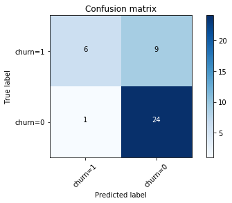
The first row is for customers whose actual churn value in the test set is 1. As you can calculate, out of 40 customers, the churn value of 15 of them is 1.A nd out of these 15, the classifier correctly predicted 6 of them as 1, and 9 of them as 0. It means that for 6 customers, the actual churn value was 1 in the test set, and the classifier correctly predicted those as 1. However, the actual label of 9 customers was 1, and the classifier predicted these as 0, which is not very good. We can consider it as the error of the model for the first row.
Let’s look at the second row. There were 25 customers for whom the churn value was 0. The classifier correctly predicted 24 of them as 0, and one of them wrongly as 1. So, it has done a good job in predicting the customers with churn value 0.
A good thing about the confusion matrix is that is shows the model’s ability to correctly predict or separate the classes.We can interpret these numbers as the count of true positives, false positives, true negatives, and false negatives.
print(classification_report(y_test, yhat)) precision recall f1-score support
0 0.73 0.96 0.83 25
1 0.86 0.40 0.55 15
accuracy 0.75 40
macro avg 0.79 0.68 0.69 40
weighted avg 0.78 0.75 0.72 40Based on the count of each section, we can calcualte precision and recall of each label. - Precision is a measure of the accuracy provided that a class label has been predicted. It is defined by: Precision = TP/(TP+FP) - Recall is the true positive rate. It is defined as: Recall = TP / (TP+FN)
So we can calculate Precision and Recall for each class.
F1 score is the harmonic average of the precision and recall, where an F1 score reaches its best value at 1 (prefect precision and recall) and worst at 0. It’s a good way to show that a classifier has a good value for both recall and precision.
Finally, we can tell the average accuracy for this classifier is the average of the F1 score for both labels, which is 0.72 in our case.
Log Loss
In Logistic regression, the output can be the probability of customer churn. Log loss measures the performance of a classifier where the predicted output is a probability between 0 and 1.
from sklearn.metrics import log_loss
log_loss(y_test, yhat_prob)
0.6017092478101187