In this blog post we will be analyzing the quality of red and white wines, and check which are the attributes that affect wine quality the most.
There are two datasets, related to red and white Vinho Verde wine samples, from the north of Portugal. The datasets can be downloaded here. The goal is to model wine quality based on physiochemical tests. Due to privacy and logistic issues, only physiochemical (inputs) and sensory (the output) variables are available (e.g. there is no data about grape types, wine brand, wine selling price, etc.).
Attribute Information:
Input variables (based on physicochemical tests): 1. fixed acidity 2. volatile acidity 3. citric acid 4. residual sugar 5. chlorides 6. free sulfur dioxide 7. total sulfur dioxide 8. density 9. pH 10. sulphates 11. alcohol
Output variable (based on sensory data): 12. quality (score between 0 and 10)
Red Wine
Let’s first consider the red wine dataset.
Data Analysis
import numpy as np
import pandas as pd
import matplotlib.pyplot as plt
%matplotlib inline
import seaborn as sns
# create a pandas dataframe
df_red = pd.read_csv('winequality-red.csv')
df_red.head()| fixed acidity | volatile acidity | citric acid | residual sugar | chlorides | free sulfur dioxide | total sulfur dioxide | density | pH | sulphates | alcohol | quality | |
|---|---|---|---|---|---|---|---|---|---|---|---|---|
| 0 | 7.4 | 0.70 | 0.00 | 1.9 | 0.076 | 11.0 | 34.0 | 0.9978 | 3.51 | 0.56 | 9.4 | 5 |
| 1 | 7.8 | 0.88 | 0.00 | 2.6 | 0.098 | 25.0 | 67.0 | 0.9968 | 3.20 | 0.68 | 9.8 | 5 |
| 2 | 7.8 | 0.76 | 0.04 | 2.3 | 0.092 | 15.0 | 54.0 | 0.9970 | 3.26 | 0.65 | 9.8 | 5 |
| 3 | 11.2 | 0.28 | 0.56 | 1.9 | 0.075 | 17.0 | 60.0 | 0.9980 | 3.16 | 0.58 | 9.8 | 6 |
| 4 | 7.4 | 0.70 | 0.00 | 1.9 | 0.076 | 11.0 | 34.0 | 0.9978 | 3.51 | 0.56 | 9.4 | 5 |
df_red.shape(1599, 12)There are 1,599 samples and 12 features, including our target feature - the wine quality.
df_red.info()<class 'pandas.core.frame.DataFrame'>
RangeIndex: 1599 entries, 0 to 1598
Data columns (total 12 columns):
# Column Non-Null Count Dtype
--- ------ -------------- -----
0 fixed acidity 1599 non-null float64
1 volatile acidity 1599 non-null float64
2 citric acid 1599 non-null float64
3 residual sugar 1599 non-null float64
4 chlorides 1599 non-null float64
5 free sulfur dioxide 1599 non-null float64
6 total sulfur dioxide 1599 non-null float64
7 density 1599 non-null float64
8 pH 1599 non-null float64
9 sulphates 1599 non-null float64
10 alcohol 1599 non-null float64
11 quality 1599 non-null int64
dtypes: float64(11), int64(1)
memory usage: 150.0 KBAll of our dataset is numeric and there are no missing values.
df_red.describe()| fixed acidity | volatile acidity | citric acid | residual sugar | chlorides | free sulfur dioxide | total sulfur dioxide | density | pH | sulphates | alcohol | quality | |
|---|---|---|---|---|---|---|---|---|---|---|---|---|
| count | 1599.000000 | 1599.000000 | 1599.000000 | 1599.000000 | 1599.000000 | 1599.000000 | 1599.000000 | 1599.000000 | 1599.000000 | 1599.000000 | 1599.000000 | 1599.000000 |
| mean | 8.319637 | 0.527821 | 0.270976 | 2.538806 | 0.087467 | 15.874922 | 46.467792 | 0.996747 | 3.311113 | 0.658149 | 10.422983 | 5.636023 |
| std | 1.741096 | 0.179060 | 0.194801 | 1.409928 | 0.047065 | 10.460157 | 32.895324 | 0.001887 | 0.154386 | 0.169507 | 1.065668 | 0.807569 |
| min | 4.600000 | 0.120000 | 0.000000 | 0.900000 | 0.012000 | 1.000000 | 6.000000 | 0.990070 | 2.740000 | 0.330000 | 8.400000 | 3.000000 |
| 25% | 7.100000 | 0.390000 | 0.090000 | 1.900000 | 0.070000 | 7.000000 | 22.000000 | 0.995600 | 3.210000 | 0.550000 | 9.500000 | 5.000000 |
| 50% | 7.900000 | 0.520000 | 0.260000 | 2.200000 | 0.079000 | 14.000000 | 38.000000 | 0.996750 | 3.310000 | 0.620000 | 10.200000 | 6.000000 |
| 75% | 9.200000 | 0.640000 | 0.420000 | 2.600000 | 0.090000 | 21.000000 | 62.000000 | 0.997835 | 3.400000 | 0.730000 | 11.100000 | 6.000000 |
| max | 15.900000 | 1.580000 | 1.000000 | 15.500000 | 0.611000 | 72.000000 | 289.000000 | 1.003690 | 4.010000 | 2.000000 | 14.900000 | 8.000000 |
To understand how much each attribute correlates with the wine quality, we can compute the standard correlation coefficient or Pearson’s r between every pair of attributes.
corr_matrix = df_red.corr()
corr_matrix['quality'].sort_values(ascending=False)
quality 1.000000
alcohol 0.476166
sulphates 0.251397
citric acid 0.226373
fixed acidity 0.124052
residual sugar 0.013732
free sulfur dioxide -0.050656
pH -0.057731
chlorides -0.128907
density -0.174919
total sulfur dioxide -0.185100
volatile acidity -0.390558
Name: quality, dtype: float64We now know the features that most affect the wine quality.
Wine quality is directly proportional to the amount of alcohol, sulphates, citric acid.
Wine quality is inversely proportional to the amount of volatile acidity, total sulfur dioxide, density.
Data Visualization
Let’s visualize the data by creating histograms and density plots. We can understand the distribution for separate attributes.
import matplotlib.pyplot as plt
%matplotlib inline
import seaborn as sns
# histograms
df_red.hist(bins=10, figsize=(20, 15))
plt.show()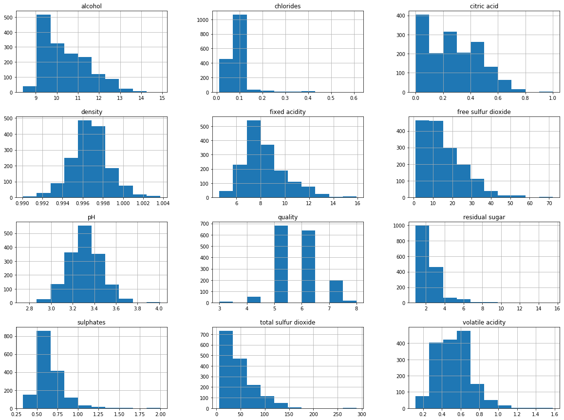
# density plots
df_red.plot(kind='density', subplots=True, figsize=(20,15),
           layout=(4,3), sharex=False)
plt.show()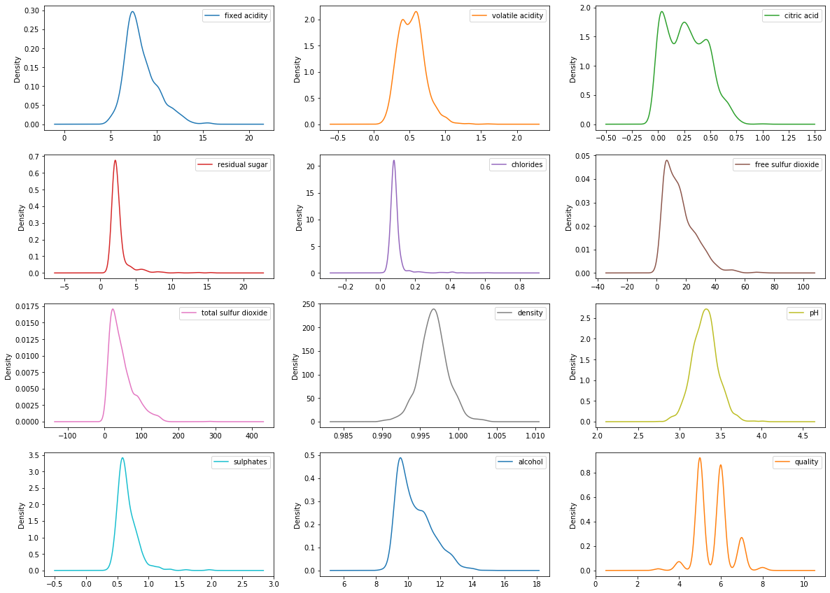
sns.distplot(df_red['quality'], hist=True, kde=True,
             bins='auto', color = 'darkblue',
             hist_kws={'edgecolor':'black'},
             kde_kws={'linewidth': 4})
plt.show()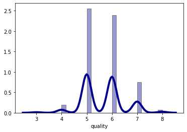
The data distribution for the alcohol, citric acid and sulfur dioxide content atrributes is positively skewed.
The data distribution for the density and pH attributes is quite normally distributed.
The wine quality data distribution is a bimodal distribution and there are more wines with an average quality than wines with good or bad quality.
from pandas.plotting import scatter_matrix
sm = scatter_matrix(df_red, figsize=(12, 12), diagonal='kde')
#Change label rotation
[s.xaxis.label.set_rotation(40) for s in sm.reshape(-1)]
[s.yaxis.label.set_rotation(0) for s in sm.reshape(-1)]
#May need to offset label when rotating to prevent overlap of figure
[s.get_yaxis().set_label_coords(-0.6,0.5) for s in sm.reshape(-1)]
#Hide all ticks
[s.set_xticks(()) for s in sm.reshape(-1)]
[s.set_yticks(()) for s in sm.reshape(-1)]
plt.show()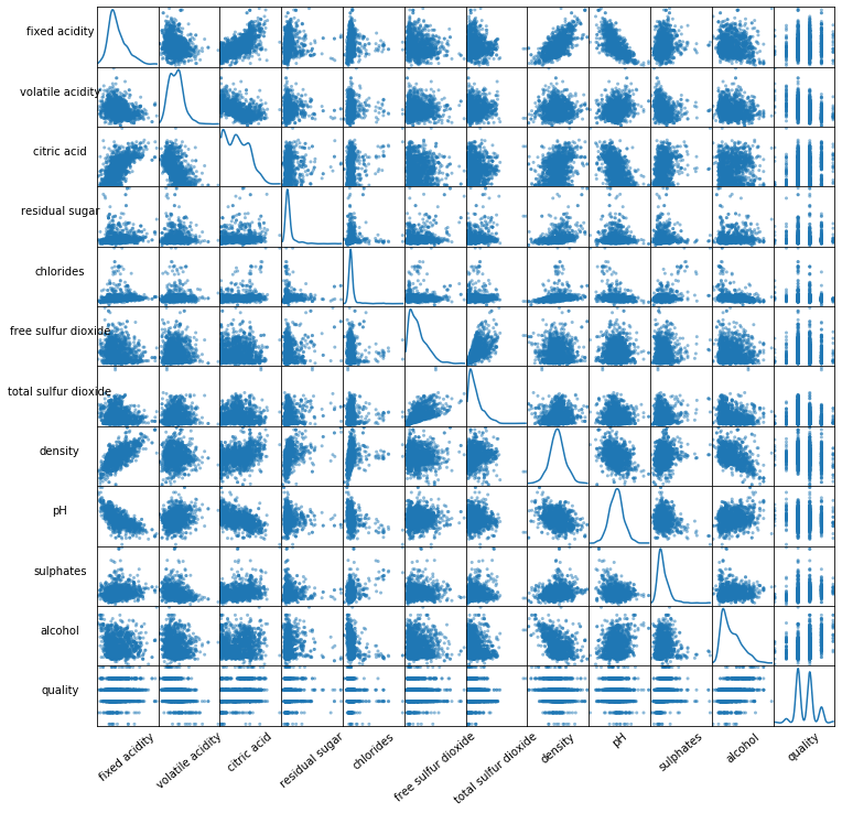
Let’s create a pivot table that describes the median value of each feature for each quality score.
# pivot table
column_names = ['fixed acidity', 'volatile acidity', 'citric acid',
                'residual sugar', 'chlorides', 'free sulfur dioxide',
                'total sulfur dioxide', 'density', 'pH', 'sulphates', 'alcohol']

df_red_pivot_table = df_red.pivot_table(column_names,
                                    ['quality'],
                                    aggfunc='median')

df_red_pivot_table| alcohol | chlorides | citric acid | density | fixed acidity | free sulfur dioxide | pH | residual sugar | sulphates | total sulfur dioxide | volatile acidity | |
|---|---|---|---|---|---|---|---|---|---|---|---|
| quality | |||||||||||
| 3 | 9.925 | 0.0905 | 0.035 | 0.997565 | 7.50 | 6.0 | 3.39 | 2.1 | 0.545 | 15.0 | 0.845 |
| 4 | 10.000 | 0.0800 | 0.090 | 0.996500 | 7.50 | 11.0 | 3.37 | 2.1 | 0.560 | 26.0 | 0.670 |
| 5 | 9.700 | 0.0810 | 0.230 | 0.997000 | 7.80 | 15.0 | 3.30 | 2.2 | 0.580 | 47.0 | 0.580 |
| 6 | 10.500 | 0.0780 | 0.260 | 0.996560 | 7.90 | 14.0 | 3.32 | 2.2 | 0.640 | 35.0 | 0.490 |
| 7 | 11.500 | 0.0730 | 0.400 | 0.995770 | 8.80 | 11.0 | 3.28 | 2.3 | 0.740 | 27.0 | 0.370 |
| 8 | 12.150 | 0.0705 | 0.420 | 0.994940 | 8.25 | 7.5 | 3.23 | 2.1 | 0.740 | 21.5 | 0.370 |
We can see just how much effect does the alcohol content and volatile acidity have on the quality of the wine.
We can plot a correlation matrix to see how two variables interact, both in direction and magnitude.
column_names = ['fixed acidity', 'volatile acidity', 'citric acid',
                'residual sugar', 'chlorides', 'free sulfur dioxide',
                'total sulfur dioxide', 'density', 'pH', 'sulphates',
                'alcohol', 'quality']

# plot correlation matrix
fig, ax = plt.subplots(figsize=(20, 20))
colormap = sns.diverging_palette(220, 10, as_cmap=True)

sns.heatmap(corr_matrix, cmap=colormap, annot=True,
           fmt='.2f', annot_kws={'size': 20})
ax.set_xticklabels(column_names,
                   rotation=45,
                   horizontalalignment='right',
                   fontsize=20);
ax.set_yticklabels(column_names, fontsize=20);
plt.show()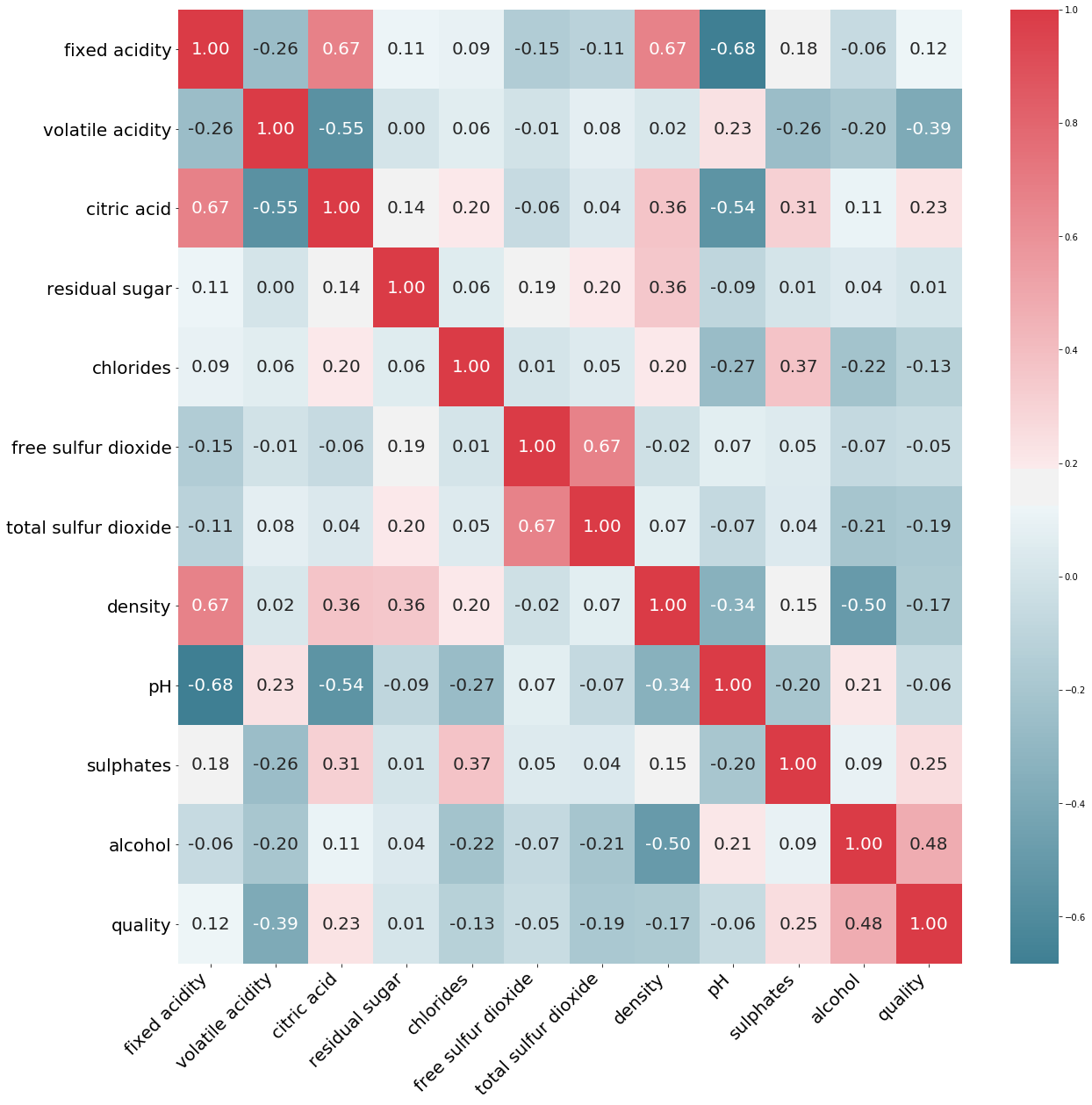
Data Cleaning
In our dataset, there aren’t any missing values, outliers, or attributes that provide no useful information for the task. So, we could conclude than our dataset is quite clean.
The wine preference scores vary from 3 to 8, so it’s straightforward to categorize them into ‘bad’ or ‘good’ quality of wines. We will assign discrete values of 0 and 1 for the corresponding categories.
# Dividing wine as good and bad by giving a limit for the quality
bins = (2, 6, 8)
group_names = ['bad', 'good']
df_red['quality'] = pd.cut(df_red['quality'], bins = bins, labels = group_names)
from sklearn.preprocessing import LabelEncoder
# let's assign labels to our quality variable
label_quality = LabelEncoder()
# Bad becomes 0 and good becomes 1
df_red['quality'] = label_quality.fit_transform(df_red['quality'])
print(df_red['quality'].value_counts())
sns.countplot(df_red['quality'])
plt.show()0 1382
1 217
Name: quality, dtype: int64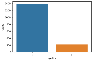
As we can see, there are far more bad quality red wines (1,382) than good quality ones (217).
Train/Test Split
Now we will split the dataset into a training set and a testing set.
# separate the dataset
X = df_red.drop('quality', axis=1)
y = df_red['quality']
from sklearn.model_selection import train_test_split
X_train, X_test, y_train, y_test = train_test_split(
X, y, test_size=0.2, random_state=42)Data Preprocessing
We will scale the features so as to get optimized results.
from sklearn.preprocessing import StandardScaler

sc = StandardScaler()
X_train = sc.fit_transform(X_train)
X_test = sc.fit_transform(X_test)
Modeling
We will be evaluating 8 different algorithms. 1. Support Vector Classifier 2. Stochastic Gradient Decent Classifier 3. Random Forest Classifier 4. Decision Tree Classifier 5. Gaussian Naive Bayes 6. K-Neighbors Classifier 7. Ada Boost Classifier 8. Logistic Regression
The key to a fair comparison of machine learning algorithms is ensuring that each algorithm is evaluated in the same way on the same data. K-fold Cross Validation provides a solution to this problem by dividing the data into folds and ensuring that each fold is used as a testing set at some point.
# import libraries
from sklearn.svm import SVC
from sklearn.linear_model import SGDClassifier
from sklearn.neighbors import KNeighborsClassifier
from sklearn.ensemble import RandomForestClassifier, AdaBoostClassifier
from sklearn.tree import DecisionTreeClassifier
from sklearn.discriminant_analysis import LinearDiscriminantAnalysis
from sklearn.naive_bayes import GaussianNB
from sklearn.linear_model import LogisticRegression
from sklearn import model_selection
from sklearn.model_selection import GridSearchCV, cross_val_score
# import warnings filter
from warnings import simplefilter
# ignore all future warnings
simplefilter(action='ignore', category=FutureWarning)# prepare configuration for cross validation test harness
seed = 7
# prepare models
models = []
models.append(('SupportVectorClassifier', SVC()))
models.append(('StochasticGradientDecentC', SGDClassifier()))
models.append(('RandomForestClassifier', RandomForestClassifier()))
models.append(('DecisionTreeClassifier', DecisionTreeClassifier()))
models.append(('GaussianNB', GaussianNB()))
models.append(('KNeighborsClassifier', KNeighborsClassifier()))
models.append(('AdaBoostClassifier', AdaBoostClassifier()))
models.append(('LogisticRegression', LogisticRegression()))# evaluate each model in turn
results = []
names = []
scoring = 'accuracy'
for name, model in models:
kfold = model_selection.KFold(n_splits=10, random_state=seed)
cv_results = model_selection.cross_val_score(model, X_train, y_train, cv=kfold, scoring=scoring)
results.append(cv_results)
names.append(name)
msg = "%s: %f (%f)" % (name, cv_results.mean(), cv_results.std())
print(msg)
# boxplot algorithm comparison
fig = plt.figure(figsize=(40, 20))
fig.suptitle('Algorithm Comparison', fontsize=40)
ax = fig.add_subplot(111)
plt.boxplot(results)
ax.set_xticklabels(names, fontdict={'fontsize': 20})
plt.show()SupportVectorClassifier: 0.889782 (0.023210)
StochasticGradientDecentC: 0.849151 (0.044240)
RandomForestClassifier: 0.912457 (0.029968)
DecisionTreeClassifier: 0.877264 (0.028120)
GaussianNB: 0.836559 (0.022781)
KNeighborsClassifier: 0.873364 (0.021081)
AdaBoostClassifier: 0.885876 (0.019715)
LogisticRegression: 0.883526 (0.031077)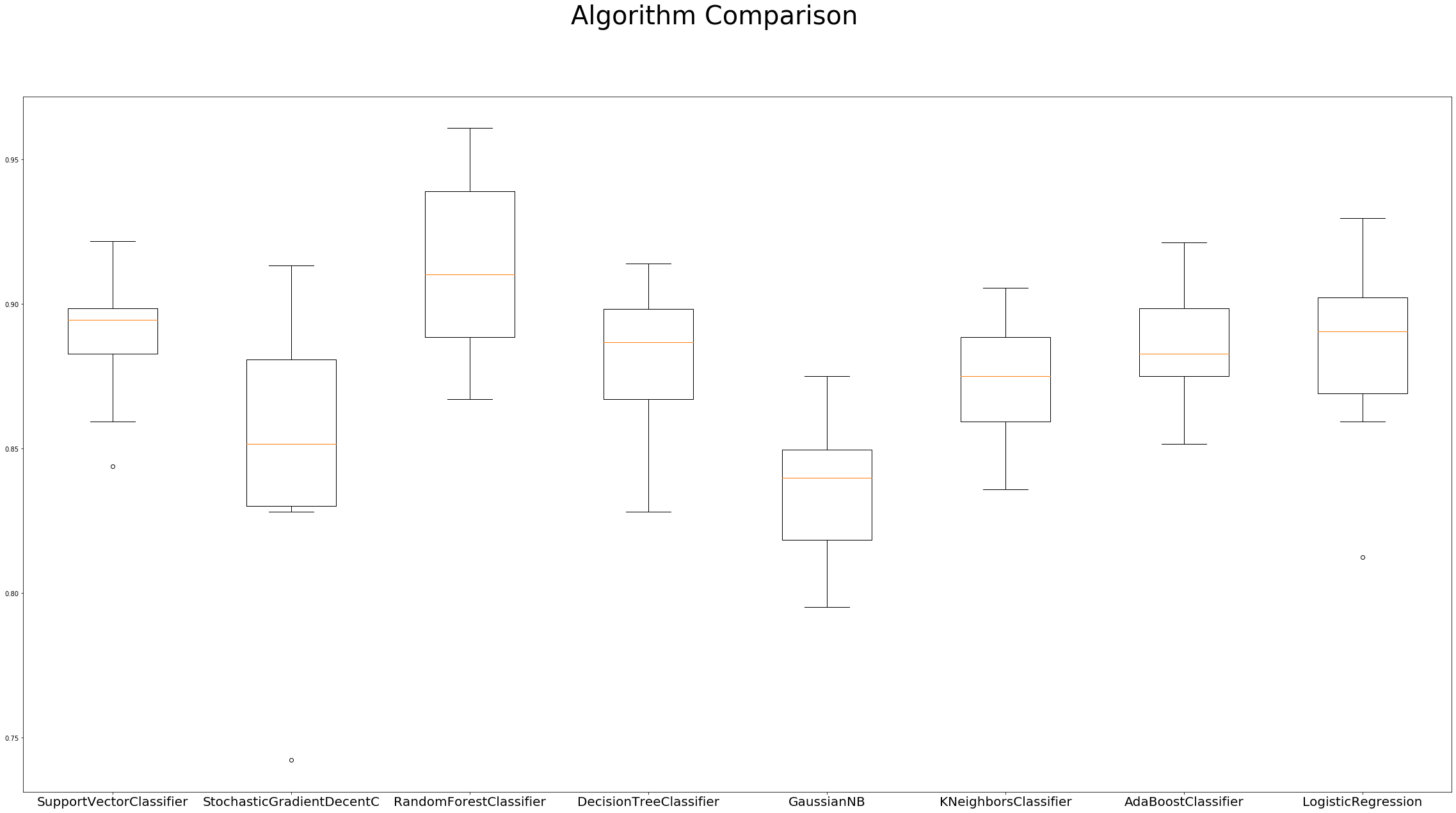
The Box Plots of these algorithms’ accuracy distribution is quite symmetrical, with negligible outliers. The adjacent box plot values are close together, which correspond to the high density of accuracy scores.
Hyperparameter Tuning
There are several factors that can help us determine which algorithm performs best. One such factor is the performance on the cross-validation set and another factor is the choice of parameters for an algorithm.
SVC
Let’s fine-tune our algorithms. The first algorithm that we trained and evaluated was the Support Vector Classifier and the mean value for model prediction was 0.889. We will use GridSearchCV for the hyperparameter tuning.
svc = SVC()
svc.fit(X_train, y_train)
pred_svc = svc.predict(X_test)def svc_param_selection(X, y, nfolds):
param = {
'C': [0.1, 0.8, 0.9, 1, 1.1, 1.2, 1.3, 1.4],
'kernel': ['linear', 'rbf'],
'gamma': [0.1, 0.8, 0.9, 1, 1.1, 1.2, 1.3, 1.4]
}
grid_search = GridSearchCV(svc, param_grid=param,
scoring='accuracy', cv=nfolds)
grid_search.fit(X, y)
return grid_search.best_params_
svc_param_selection(X_train, y_train, 10){'C': 1.2, 'gamma': 0.9, 'kernel': 'rbf'}Hence, the best parameters for the SVC algorithm are {C= 1.2, gamma= 0.9 , kernel= rbf}.
Let’s run our SVC algorithm again with the best parameters.
from sklearn.metrics import confusion_matrix, classification_report, accuracy_score, mean_absolute_error
svc2 = SVC(C= 1.2, gamma= 0.9, kernel= 'rbf')
svc2.fit(X_train, y_train)
pred_svc2 = svc2.predict(X_test)
print('Confusion matrix')
print(confusion_matrix(y_test, pred_svc2))
print('Classification report')
print(classification_report(y_test, pred_svc2))
print('Accuracy score',accuracy_score(y_test, pred_svc2))Confusion matrix
[[271 2]
[ 31 16]]
Classification report
precision recall f1-score support
0 0.90 0.99 0.94 273
1 0.89 0.34 0.49 47
accuracy 0.90 320
macro avg 0.89 0.67 0.72 320
weighted avg 0.90 0.90 0.88 320
Accuracy score 0.896875The overall accuracy of the classifier is 89.69%, and f1-score of the weighted avg is 0.88, which is very good.
Stochastic Gradient Descent Classifier
sgd = SGDClassifier(loss='hinge', penalty='l2', max_iter=60)
sgd.fit(X_train, y_train)
pred_sgd = sgd.predict(X_test)Random Forest Classifier
rfc = RandomForestClassifier(n_estimators=200, max_depth=20,
random_state=0)
rfc.fit(X_train, y_train)
pred_rfc = rfc.predict(X_test)KNeighbors Classifier
knn = KNeighborsClassifier()
knn.fit(X_train, y_train)
pred_knn = knn.predict(X_test)def knn_param_selection(X, y, nfolds):
param = {
'n_neighbors': [2, 3, 4, 5, 6],
'weights': ['uniform', 'distance'],
'algorithm': ['auto', 'ball_tree', 'kd_tree', 'brute'],
'p': [1, 2]
}
grid_search = GridSearchCV(knn, param_grid=param,
scoring='accuracy', cv=nfolds)
grid_search.fit(X, y)
return grid_search.best_params_
knn_param_selection(X_train, y_train, 10){'algorithm': 'auto', 'n_neighbors': 4, 'p': 2, 'weights': 'distance'}Hence, the best parameters for the KNeighborsClassifier algorithm are {algorithm= auto, n_neighbors= 4 , p= 2, weights= distance}.
Let’s run our knn algorithm again with the best parameters.
knn2 = KNeighborsClassifier(algorithm= 'auto',
n_neighbors= 5, p=2,
weights='distance')
knn2.fit(X_train, y_train)
pred_knn2 = knn2.predict(X_test)
print('Confusion matrix')
print(confusion_matrix(y_test, pred_knn2))
print('Classification report')
print(classification_report(y_test, pred_knn2))
print('Accuracy score',accuracy_score(y_test, pred_knn2))Confusion matrix
[[261 12]
[ 19 28]]
Classification report
precision recall f1-score support
0 0.93 0.96 0.94 273
1 0.70 0.60 0.64 47
accuracy 0.90 320
macro avg 0.82 0.78 0.79 320
weighted avg 0.90 0.90 0.90 320
Accuracy score 0.903125The overall accuracy of the classifier is 90.3%, and f1-score of the weighted avg is 0.90, which is very good.
AdaBoost Classifier
ada_classifier = AdaBoostClassifier(n_estimators=100)
ada_classifier.fit(X_train, y_train)
pred_ada = ada_classifier.predict(X_test)# cross validation
scores = cross_val_score(ada_classifier,X_test,y_test, cv=5)
print('Accuracy score',scores.mean())Accuracy score 0.84375Model Evaluation
We can compare the models by calculating their mean absolute error and accuracy.
def evaluate(model, test_features, test_labels):
predictions = model.predict(test_features)
print('Model Performance')
print('Average Error: {:0.4f} degrees.'.format(
mean_absolute_error(test_labels, predictions)))
print('Accuracy = {:0.2f}%.'.format(accuracy_score(
test_labels, predictions)*100))evaluate(svc,X_test,y_test)
evaluate(svc2,X_test,y_test)
evaluate(sgd,X_test,y_test)
evaluate(rfc,X_test,y_test)
evaluate(knn2, X_test, y_test)
evaluate(ada_classifier,X_test,y_test)Model Performance
Average Error: 0.1250 degrees.
Accuracy = 87.50%.
Model Performance
Average Error: 0.1031 degrees.
Accuracy = 89.69%.
Model Performance
Average Error: 0.1688 degrees.
Accuracy = 83.12%.
Model Performance
Average Error: 0.1125 degrees.
Accuracy = 88.75%.
Model Performance
Average Error: 0.0969 degrees.
Accuracy = 90.31%.
Model Performance
Average Error: 0.1594 degrees.
Accuracy = 84.06%.The KNeighborsClassifier model with hyperparameter tuning performs the best with an accuracy of 90.31%.
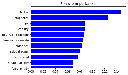
Feature Importance
We could also analyze the feature importance for an algorithm.
importance = rfc.feature_importances_
std = np.std([tree.feature_importances_ for tree in rfc.estimators_],
axis=0)
indices = np.argsort(importance)
# plot the feature importances of the forest
plt.figure()
plt.title("Feature importances")
plt.barh(range(X.shape[1]), importance[indices],
color="b", align="center")
plt.yticks(range(X.shape[1]), column_names)
plt.ylim([0, X.shape[1]])
plt.show()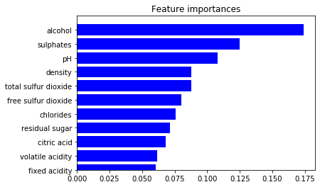
White Wine
Let us now consider the white wine dataset.
# create a pandas dataframe
df_white = pd.read_csv('winequality-white.csv')
df_white.head()| fixed acidity | volatile acidity | citric acid | residual sugar | chlorides | free sulfur dioxide | total sulfur dioxide | density | pH | sulphates | alcohol | quality | |
|---|---|---|---|---|---|---|---|---|---|---|---|---|
| 0 | 7.0 | 0.27 | 0.36 | 20.7 | 0.045 | 45.0 | 170.0 | 1.0010 | 3.00 | 0.45 | 8.8 | 6 |
| 1 | 6.3 | 0.30 | 0.34 | 1.6 | 0.049 | 14.0 | 132.0 | 0.9940 | 3.30 | 0.49 | 9.5 | 6 |
| 2 | 8.1 | 0.28 | 0.40 | 6.9 | 0.050 | 30.0 | 97.0 | 0.9951 | 3.26 | 0.44 | 10.1 | 6 |
| 3 | 7.2 | 0.23 | 0.32 | 8.5 | 0.058 | 47.0 | 186.0 | 0.9956 | 3.19 | 0.40 | 9.9 | 6 |
| 4 | 7.2 | 0.23 | 0.32 | 8.5 | 0.058 | 47.0 | 186.0 | 0.9956 | 3.19 | 0.40 | 9.9 | 6 |
df_white.shape(4898, 12)There are 4,898 samples and 12 features, including our target feature - the wine quality.
df_white.info()<class 'pandas.core.frame.DataFrame'>
RangeIndex: 4898 entries, 0 to 4897
Data columns (total 12 columns):
# Column Non-Null Count Dtype
--- ------ -------------- -----
0 fixed acidity 4898 non-null float64
1 volatile acidity 4898 non-null float64
2 citric acid 4898 non-null float64
3 residual sugar 4898 non-null float64
4 chlorides 4898 non-null float64
5 free sulfur dioxide 4898 non-null float64
6 total sulfur dioxide 4898 non-null float64
7 density 4898 non-null float64
8 pH 4898 non-null float64
9 sulphates 4898 non-null float64
10 alcohol 4898 non-null float64
11 quality 4898 non-null int64
dtypes: float64(11), int64(1)
memory usage: 459.3 KBdf_white.describe()| fixed acidity | volatile acidity | citric acid | residual sugar | chlorides | free sulfur dioxide | total sulfur dioxide | density | pH | sulphates | alcohol | quality | |
|---|---|---|---|---|---|---|---|---|---|---|---|---|
| count | 4898.000000 | 4898.000000 | 4898.000000 | 4898.000000 | 4898.000000 | 4898.000000 | 4898.000000 | 4898.000000 | 4898.000000 | 4898.000000 | 4898.000000 | 4898.000000 |
| mean | 6.854788 | 0.278241 | 0.334192 | 6.391415 | 0.045772 | 35.308085 | 138.360657 | 0.994027 | 3.188267 | 0.489847 | 10.514267 | 5.877909 |
| std | 0.843868 | 0.100795 | 0.121020 | 5.072058 | 0.021848 | 17.007137 | 42.498065 | 0.002991 | 0.151001 | 0.114126 | 1.230621 | 0.885639 |
| min | 3.800000 | 0.080000 | 0.000000 | 0.600000 | 0.009000 | 2.000000 | 9.000000 | 0.987110 | 2.720000 | 0.220000 | 8.000000 | 3.000000 |
| 25% | 6.300000 | 0.210000 | 0.270000 | 1.700000 | 0.036000 | 23.000000 | 108.000000 | 0.991723 | 3.090000 | 0.410000 | 9.500000 | 5.000000 |
| 50% | 6.800000 | 0.260000 | 0.320000 | 5.200000 | 0.043000 | 34.000000 | 134.000000 | 0.993740 | 3.180000 | 0.470000 | 10.400000 | 6.000000 |
| 75% | 7.300000 | 0.320000 | 0.390000 | 9.900000 | 0.050000 | 46.000000 | 167.000000 | 0.996100 | 3.280000 | 0.550000 | 11.400000 | 6.000000 |
| max | 14.200000 | 1.100000 | 1.660000 | 65.800000 | 0.346000 | 289.000000 | 440.000000 | 1.038980 | 3.820000 | 1.080000 | 14.200000 | 9.000000 |
corr_matrix2 = df_white.corr()
corr_matrix2['quality'].sort_values(ascending=False)quality 1.000000
alcohol 0.435575
pH 0.099427
sulphates 0.053678
free sulfur dioxide 0.008158
citric acid -0.009209
residual sugar -0.097577
fixed acidity -0.113663
total sulfur dioxide -0.174737
volatile acidity -0.194723
chlorides -0.209934
density -0.307123
Name: quality, dtype: float64The features that have the biggest impact on wine quality are alcohol, pH, sulphates, chlorides, density, and volatile acidity.
Data Visualization
# histograms
df_white.hist(bins=10, figsize=(20, 15))
plt.show()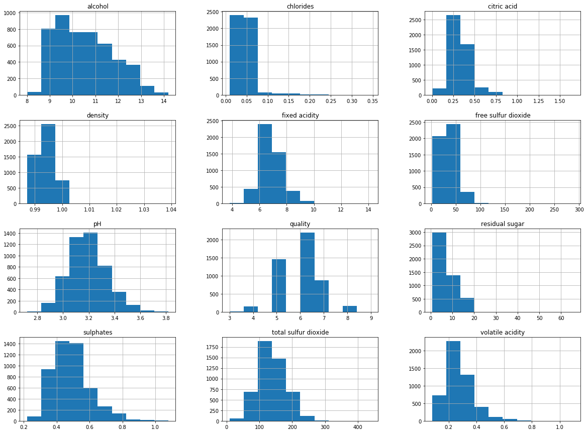
# pivot table
column_names = ['fixed acidity', 'volatile acidity', 'citric acid',
'residual sugar', 'chlorides', 'free sulfur dioxide',
'total sulfur dioxide', 'density', 'pH', 'sulphates', 'alcohol']
df_white_pivot_table = df_white.pivot_table(column_names,
['quality'],
aggfunc='median')
df_white_pivot_table| alcohol | chlorides | citric acid | density | fixed acidity | free sulfur dioxide | pH | residual sugar | sulphates | total sulfur dioxide | volatile acidity | |
|---|---|---|---|---|---|---|---|---|---|---|---|
| quality | |||||||||||
| 3 | 10.45 | 0.041 | 0.345 | 0.994425 | 7.3 | 33.5 | 3.215 | 4.60 | 0.44 | 159.5 | 0.26 |
| 4 | 10.10 | 0.046 | 0.290 | 0.994100 | 6.9 | 18.0 | 3.160 | 2.50 | 0.47 | 117.0 | 0.32 |
| 5 | 9.50 | 0.047 | 0.320 | 0.995300 | 6.8 | 35.0 | 3.160 | 7.00 | 0.47 | 151.0 | 0.28 |
| 6 | 10.50 | 0.043 | 0.320 | 0.993660 | 6.8 | 34.0 | 3.180 | 5.30 | 0.48 | 132.0 | 0.25 |
| 7 | 11.40 | 0.037 | 0.310 | 0.991760 | 6.7 | 33.0 | 3.200 | 3.65 | 0.48 | 122.0 | 0.25 |
| 8 | 12.00 | 0.036 | 0.320 | 0.991640 | 6.8 | 35.0 | 3.230 | 4.30 | 0.46 | 122.0 | 0.26 |
| 9 | 12.50 | 0.031 | 0.360 | 0.990300 | 7.1 | 28.0 | 3.280 | 2.20 | 0.46 | 119.0 | 0.27 |
# density plots
df_white.plot(kind='density', subplots=True, figsize=(20,15),
layout=(4,3), sharex=False)
plt.show()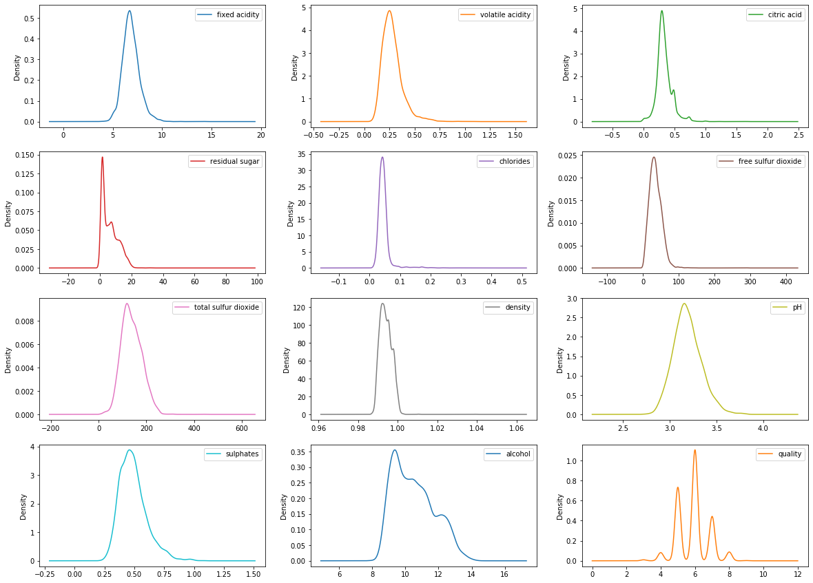
sns.distplot(df_white['quality'], hist=True, kde=True,
bins='auto', color = 'darkblue',
hist_kws={'edgecolor':'black'},
kde_kws={'linewidth': 4})
plt.show()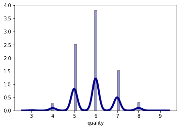
from pandas.plotting import scatter_matrix
sm = scatter_matrix(df_white, figsize=(12, 12), diagonal='kde')
#Change label rotation
[s.xaxis.label.set_rotation(40) for s in sm.reshape(-1)]
[s.yaxis.label.set_rotation(0) for s in sm.reshape(-1)]
#May need to offset label when rotating to prevent overlap of figure
[s.get_yaxis().set_label_coords(-0.6,0.5) for s in sm.reshape(-1)]
#Hide all ticks
[s.set_xticks(()) for s in sm.reshape(-1)]
[s.set_yticks(()) for s in sm.reshape(-1)]
plt.show()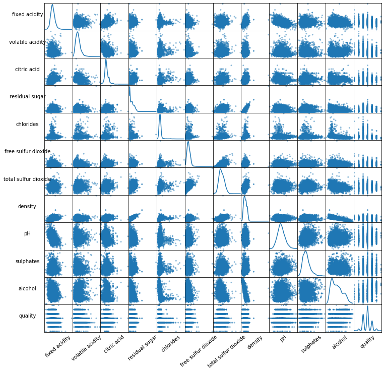
column_names = ['fixed acidity', 'volatile acidity', 'citric acid',
'residual sugar', 'chlorides', 'free sulfur dioxide',
'total sulfur dioxide', 'density', 'pH', 'sulphates',
'alcohol', 'quality']
# plot correlation matrix
fig, ax = plt.subplots(figsize=(20, 20))
colormap = sns.diverging_palette(220, 10, as_cmap=True)
sns.heatmap(corr_matrix2, cmap=colormap, annot=True,
fmt='.2f', annot_kws={'size': 20})
ax.set_xticklabels(column_names,
rotation=45,
horizontalalignment='right',
fontsize=20);
ax.set_yticklabels(column_names, fontsize=20);
plt.show()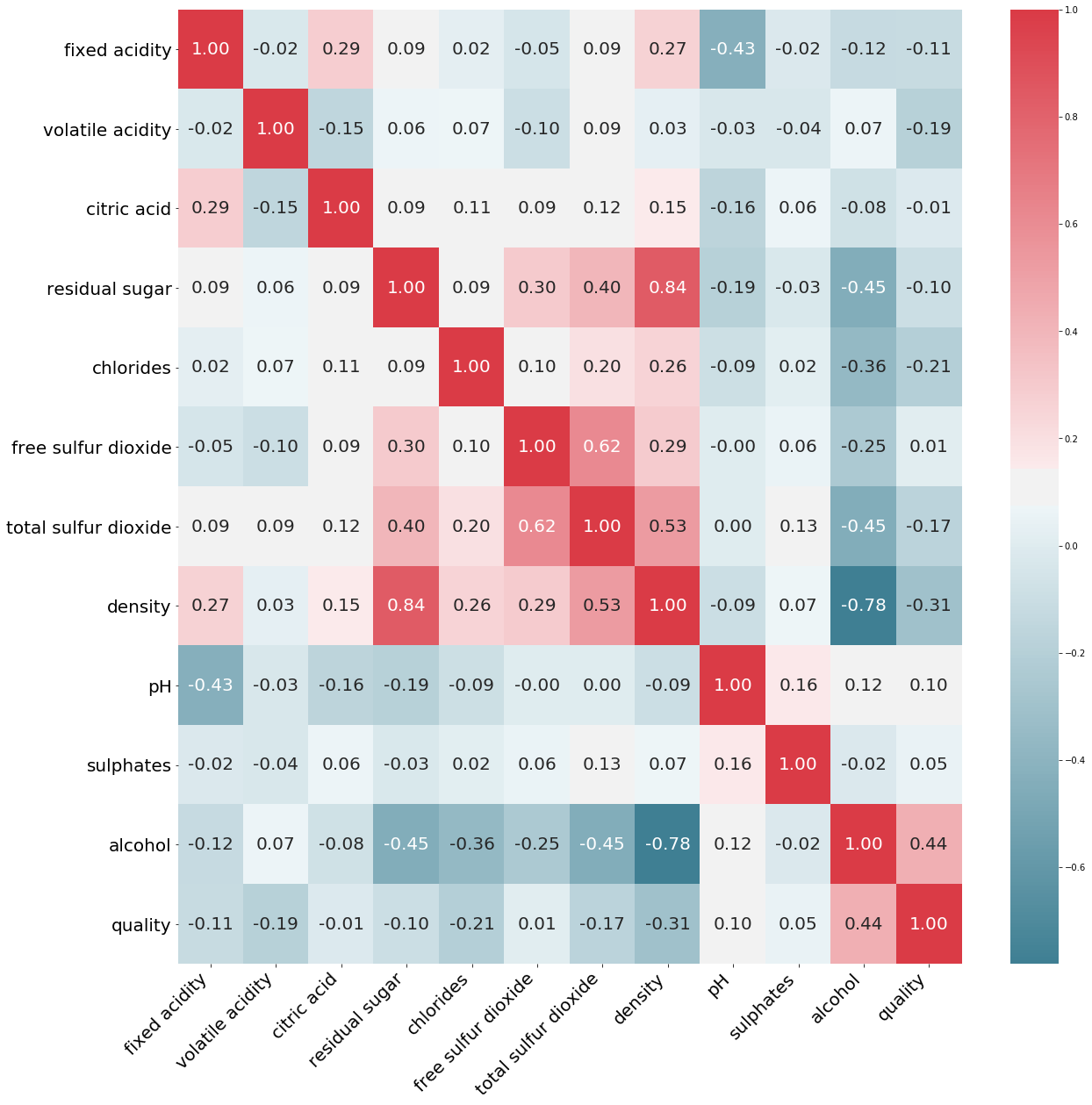
# Dividing wine as good and bad by giving a limit for the quality
bins = (2, 6, 9)
group_names = ['bad', 'good']
df_white['quality'] = pd.cut(df_white['quality'], bins = bins, labels = group_names)# let's assign labels to our quality variable
label_quality = LabelEncoder()
# Bad becomes 0 and good becomes 1
df_white['quality'] = label_quality.fit_transform(df_white['quality'])
print(df_white['quality'].value_counts())
sns.countplot(df_white['quality'])
plt.show()0 3838
1 1060
Name: quality, dtype: int64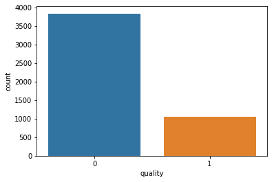
There are 3,838 bad quality wines, and 1,060 good quality wines.
Train/Test Split
# separate the dataset
X = df_white.drop('quality', axis=1)
y = df_white['quality']X_train, X_test, y_train, y_test = train_test_split(
X, y, test_size=0.2, random_state=42)Data Preprocessing
from sklearn.preprocessing import StandardScaler
sc = StandardScaler()
X_train = sc.fit_transform(X_train)
X_test = sc.fit_transform(X_test)Modeling
# prepare configuration for cross validation test harness
seed = 7
# prepare models
models = []
models.append(('SupportVectorClassifier', SVC()))
models.append(('StochasticGradientDecentC', SGDClassifier()))
models.append(('RandomForestClassifier', RandomForestClassifier()))
models.append(('DecisionTreeClassifier', DecisionTreeClassifier()))
models.append(('GaussianNB', GaussianNB()))
models.append(('KNeighborsClassifier', KNeighborsClassifier()))
models.append(('AdaBoostClassifier', AdaBoostClassifier()))
models.append(('LogisticRegression', LogisticRegression()))# evaluate each model in turn
results = []
names = []
scoring = 'accuracy'
for name, model in models:
   kfold = model_selection.KFold(n_splits=10, random_state=seed)
   cv_results = model_selection.cross_val_score(model, X_train, y_train, cv=kfold, scoring=scoring)
   results.append(cv_results)
   names.append(name)
   msg = "%s: %f (%f)" % (name, cv_results.mean(), cv_results.std())
   print(msg)

# boxplot algorithm comparison
fig = plt.figure(figsize=(40, 20))
fig.suptitle('Algorithm Comparison', fontsize=40)
ax = fig.add_subplot(111)
plt.boxplot(results)
ax.set_xticklabels(names, fontdict={'fontsize': 20})
plt.show()
SupportVectorClassifier: 0.825930 (0.020147)
StochasticGradientDecentC: 0.789953 (0.023700)
RandomForestClassifier: 0.874421 (0.014710)
DecisionTreeClassifier: 0.818526 (0.019489)
GaussianNB: 0.729720 (0.029256)
KNeighborsClassifier: 0.830781 (0.018867)
AdaBoostClassifier: 0.818019 (0.017404)
LogisticRegression: 0.804491 (0.017744)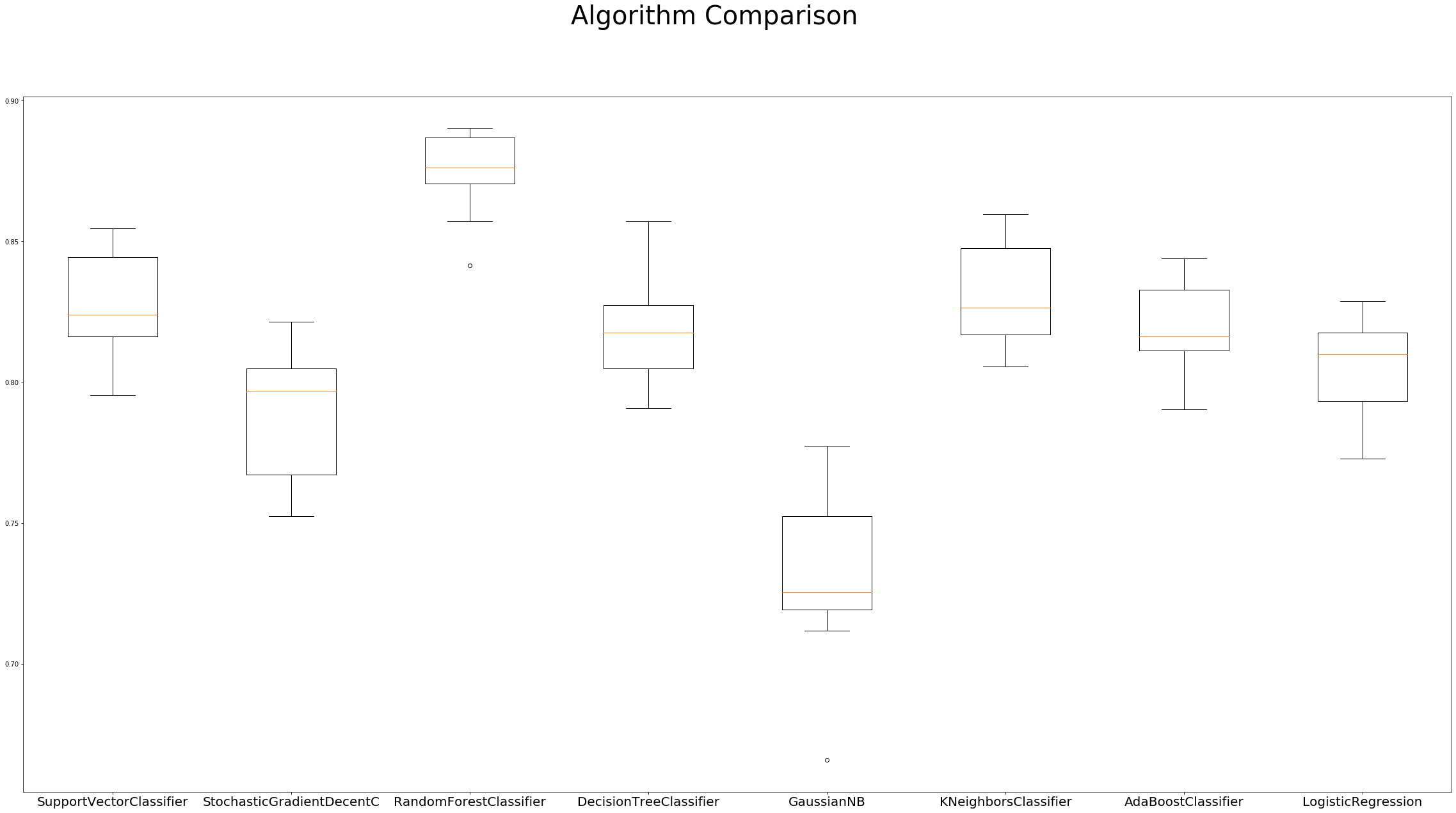
Hyperparameter Tuning
SVC
svc = SVC()
svc.fit(X_train, y_train)
pred_svc = svc.predict(X_test)
def svc_param_selection(X, y, nfolds):
param = {
'C': [0.1, 0.8, 0.9, 1, 1.1, 1.2, 1.3, 1.4],
'kernel': ['linear', 'rbf'],
'gamma': [0.1, 0.8, 0.9, 1, 1.1, 1.2, 1.3, 1.4]
}
grid_search = GridSearchCV(svc, param_grid=param,
scoring='accuracy', cv=nfolds)
grid_search.fit(X, y)
return grid_search.best_params_
svc_param_selection(X_train, y_train, 10){'C': 1.4, 'gamma': 1.1, 'kernel': 'rbf'}from sklearn.metrics import confusion_matrix, classification_report, accuracy_score, mean_absolute_error
svc2 = SVC(C= 1.4, gamma= 1.1, kernel= 'rbf')
svc2.fit(X_train, y_train)
pred_svc2 = svc2.predict(X_test)
print('Confusion matrix')
print(confusion_matrix(y_test, pred_svc2))
print('Classification report')
print(classification_report(y_test, pred_svc2))
print('Accuracy score',accuracy_score(y_test, pred_svc2))Confusion matrix
[[730 23]
[103 124]]
Classification report
precision recall f1-score support
0 0.88 0.97 0.92 753
1 0.84 0.55 0.66 227
accuracy 0.87 980
macro avg 0.86 0.76 0.79 980
weighted avg 0.87 0.87 0.86 980
Accuracy score 0.8714285714285714SGD Classifier
sgd = SGDClassifier(loss='hinge', penalty='l2', max_iter=60)
sgd.fit(X_train, y_train)
pred_sgd = sgd.predict(X_test)
Random Forest Classifier
rfc = RandomForestClassifier(n_estimators=200, max_depth=20,
                             random_state=0)
rfc.fit(X_train, y_train)
pred_rfc = rfc.predict(X_test)
KNeighbors Classifier
knn = KNeighborsClassifier()
knn.fit(X_train, y_train)
pred_knn = knn.predict(X_test)
def knn_param_selection(X, y, nfolds):
param = {
'n_neighbors': [2, 3, 4, 5, 6],
'weights': ['uniform', 'distance'],
'algorithm': ['auto', 'ball_tree', 'kd_tree', 'brute'],
'p': [1, 2]
}
grid_search = GridSearchCV(knn, param_grid=param,
scoring='accuracy', cv=nfolds)
grid_search.fit(X, y)
return grid_search.best_params_
knn_param_selection(X_train, y_train, 10){'algorithm': 'auto', 'n_neighbors': 6, 'p': 1, 'weights': 'distance'}knn2 = KNeighborsClassifier(algorithm= 'auto',
n_neighbors= 5, p=2,
weights='distance')
knn2.fit(X_train, y_train)
pred_knn2 = knn2.predict(X_test)
print('Confusion matrix')
print(confusion_matrix(y_test, pred_knn2))
print('Classification report')
print(classification_report(y_test, pred_knn2))
print('Accuracy score',accuracy_score(y_test, pred_knn2))Confusion matrix
[[708 45]
[ 75 152]]
Classification report
precision recall f1-score support
0 0.90 0.94 0.92 753
1 0.77 0.67 0.72 227
accuracy 0.88 980
macro avg 0.84 0.80 0.82 980
weighted avg 0.87 0.88 0.87 980
Accuracy score 0.8775510204081632AdaBoost Classifier
ada_classifier = AdaBoostClassifier(n_estimators=100)
ada_classifier.fit(X_train, y_train)
pred_ada = ada_classifier.predict(X_test)
# cross validation
scores = cross_val_score(ada_classifier,X_test,y_test, cv=5)
print('Accuracy score',scores.mean())Accuracy score 0.7704081632653061Model Evaluation
def evaluate(model, test_features, test_labels):
    predictions = model.predict(test_features)
    print('Model Performance')
    print('Average Error: {:0.4f} degrees.'.format(
        mean_absolute_error(test_labels, predictions)))
    print('Accuracy = {:0.2f}%.'.format(accuracy_score(
test_labels, predictions)*100))Feature Importance
evaluate(svc,X_test,y_test)
evaluate(svc2,X_test,y_test)
evaluate(sgd,X_test,y_test)
evaluate(rfc,X_test,y_test)
evaluate(knn2, X_test, y_test)
evaluate(ada_classifier,X_test,y_test)
Model Performance
Average Error: 0.1796 degrees.
Accuracy = 82.04%.
Model Performance
Average Error: 0.1286 degrees.
Accuracy = 87.14%.
Model Performance
Average Error: 0.2235 degrees.
Accuracy = 77.65%.
Model Performance
Average Error: 0.1276 degrees.
Accuracy = 87.24%.
Model Performance
Average Error: 0.1224 degrees.
Accuracy = 87.76%.
Model Performance
Average Error: 0.2071 degrees.
Accuracy = 79.29%.importance = rfc.feature_importances_
std = np.std([tree.feature_importances_ for tree in rfc.estimators_],
axis=0)
indices = np.argsort(importance)
# plot the feature importances of the forest
plt.figure()
plt.title("Feature importances")
plt.barh(range(X.shape[1]), importance[indices],
color="b", align="center")
plt.yticks(range(X.shape[1]), column_names)
plt.ylim([0, X.shape[1]])
plt.show()